Advanced Practical Chemistry - Part II

After the introduction to molecular dynamics in week 1, the students were unleased on their own mini-research project - investigating the transport properties of CaF₂. In this exercise, we wanted the students to user DL_POLY to determine the temperature range within which CaF₂ becomes a fast ion conductor. For context, CaF₂ is already well studied and was choosen because the literature is full of examples for students to compare their results against.

Week 2

This week, and the subsequent two weeks, aim to put emphasis on the transport properties of materials and on how to analyse the large quantities of data produces by MD simulations. The transport properties of a material are important in many modern technological applications. For example, solid oxide fuel cells (SOFCs - alternatives to traditional batteries) are dependent on the movement of charge carriers through the solid electrolyte and nuclear fuel materials oxidise and fall apart and this corrosive behaviour is dependent on the diffusion of oxygen into the lattice. Due to the importance of the transport properties of these materials, scientists and engineers spend large amounts of their time trying to optimise these properties.

The week began with a background tutorial in how to use DL_POLY within a Jupyter Notebook. In this way, we could provide the instruction in Markdown cells, and then the DL_POLY simulations could be launched with a subprocess call in the following code cell. This would eliminate the need for a traditional, printed lab manual.

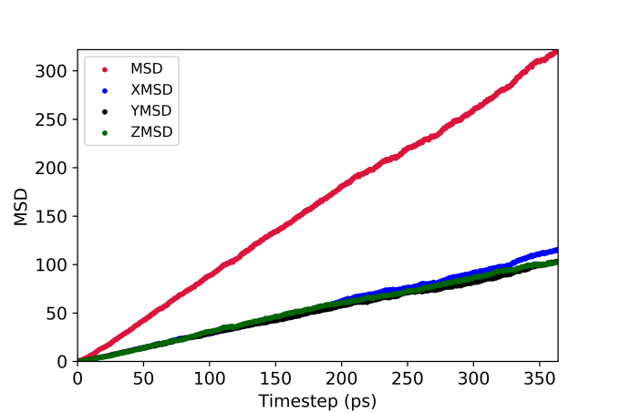
Transport properties are the end game of the exercise, so it is important to show the students how to analyses their data in order to obtain diffusion coefficients and what these quantities actually mean. DL_POLY prints out a diffusion coefficient, but this is useless in a learning environment because the students need to understand where the number comes from. So a theoretical background was provided in Markdown cells explaining mean squared displacements (MSD) and Arrhenius plots.

The final part of the tutorial, before the students we set loose, to determine the fast ion conduction temperature range in CaF₂ was to show them how to analyse their data. A few months ago, as a learning/procrastination exercise, I wrote an MSD analysis code for DL_POLY, so the students were given a stripped down version to use for analysis. The general workflow looks like this.

data = msd.read_history("Example/HISTORY", "F") msd_data = msd.run_msd(data)

plt.plot(msd_data['time'], msd_data['msd'], lw=2, color="red", label="MSD")
plt.plot(msd_data['time'], msd_data['xmsd'], lw=2, color="blue", label="X-MSD")
plt.plot(msd_data['time'], msd_data['ymsd'], lw=2, color="green", label="Y-MSD")
plt.plot(msd_data['time'], msd_data['zmsd'], lw=2, color="black", label="Z-MSD")

plt.ylabel("MSD (" r'$\AA$' ")", fontsize=15)
plt.xlabel("Time / ps", fontsize=15)
plt.ylim(0, np.amax(msd_data['msd']))
plt.xlim(0, np.amax(msd_data['time']))
plt.legend(loc=2, frameon=False)
plt.show()

​

slope, intercept, r_value, p_value, std_err = stats.linregress(msd_data['time'], msd_data['msd'])

diffusion_coefficient = (np.average(slope) / 6)
print("Diffusion Coefficient: ", diffusion_coefficient, " X 10 ^-9 (m/s^-2)")

Diffusion Coefficient: 1.4550282026323467 X 10 ^-9 (m/s^-2)

And that was it.

It took them about an hour to get through the full tutorial and then they were free to run theiry own simulations at various temperatures. For me, it proved to be an interesting teaching experiment. In order to analyse their data they had two options, they could open the DL_POLY output and copy the diffusion coefficient to an Excel spreadsheet, or they could use the method outlined above and analyse their simulations programmatically in a single notebook. I was pleased to note that nearly everyone used the latter method, for a variety of reasons:

1. The students were required to keep a hand-written lab book to ensure reproducibility (sigh). Students would record everything that they did and then a member of staff would grade it based upon how likely it is that they could repeat their work. Some of the students quickly deduced that by running everything in a notebook, they could provide their simulation data along with the notebook and by definition of the mark scheme…get full marks.
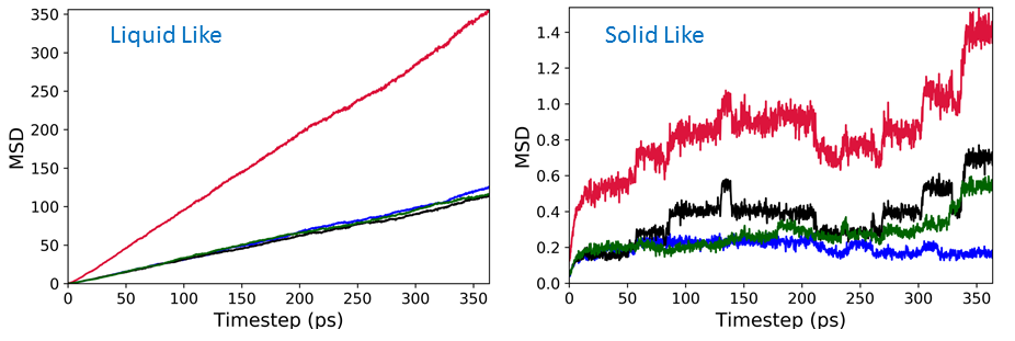
2. The MSD plot shown above can reveal an awful lot about the behaviour of the system. For example, the figure below compares the MSD for fluorine at 1500 K (left) and 300 K (right). It is easy to tell from these the state of the system.
3. Simplicity. Some students ran 30+ simulations and quickly realised that opening the large output file, searching for the diffusion coefficient and then copying it to excel is incredibly boring and tedious.

​

Feedback

In the past, we have run this lab without the Python based tutorials, or the introduction to molecular dynamics. I remember last year being asked by two students why they had both run the same simulation but got slightly different diffusion coefficients. I have to explain what MD was and that the initial velocities were assigned randomly, thus their answeres would be slightly different. When asked the same question this year, my answer was simply “think back to last week”, and within 15 seconds this was met with “Oh yeah! The velocities are randomly assigned”. So the introduction to MD in week 1 was clearly a success.

Feedback this week was largely positive, there were issues at the beginning with setting up file-paths to the DL_POLY code, this may need to be addressed in future years as it was clear that file-paths go beyond some students understanding. In contrast to last year, much les time was devoted to copying diffusion coefficients from an output file to a spreadsheet and much more time was spent actually thinking about the data collected. The students who has not dabbled with Python before week 1 had no issues with the programming in week 2 and were able to use the analysis code without any difficulty. In future years, I think that the programming can be expanded further and they would be able to write their own bits of analysis, for example they were given the above snippet, however I believe that many could write it themselves without any difficulty.

In week 3 the students will be taking on Frenkel and Schottky defects - stay tuned.