
Geometry Optimisation#
Stationary points#
Chemists are often interested in finding stationary points on potential energy surfaces.
Stationary points are points where the gradient of the potential energy surface is zero.
i.e., in one dimension
In higher dimensions we require all the partial derivatives to be zero:
where \(\alpha\) runs over all degrees of freedom.
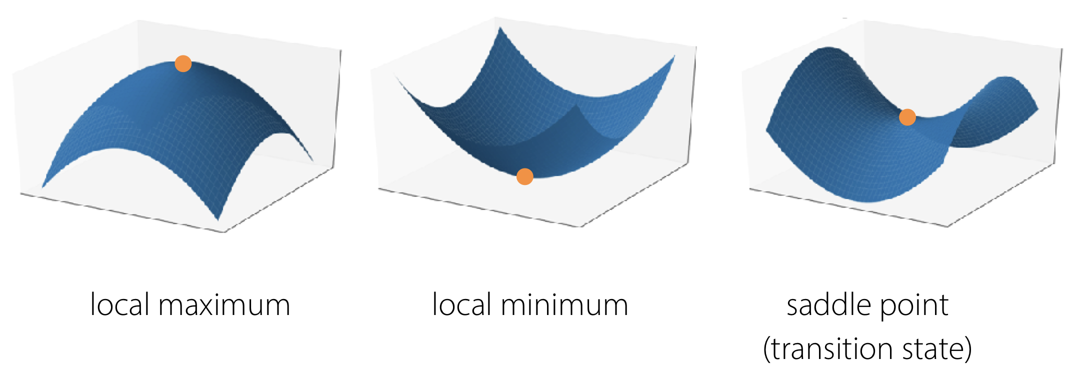
Stationary points can be minima, saddle points, or maxima.
Why do we care about stationary points?#
Remember that every point on a potential energy surface corresponds to specific atomic geometry. Stationary points correspond to specific geometries that are often particularly important in a chemsitry context:
Minima correspond to equilibrium geometries of reactants, products, or intermediates.
The global minimum gives the thermodynamic product.
Local minima give metastable products or intermediates.
The relative energies of various minima give the difference in potential energies between e.g. reactants and products.
Saddle points correspond to a transition state between the two adjacent minima.
Finding the saddle point gives us the transition state geometry.
The energy difference between the transition state and the adjacent potential energy minimum, corresponding to the reactants, gives the energy barrier along the reaction coordinate for a chemical process.
Note that we cannot have saddle-points on a one-dimensional potential energy surface.
Maxima are often less relevant to understanding chemical behaviour.
If we consider the complete potential energy surface then we will have a number of poorly defined “maxima” with infinite energy, corresponding to atoms sitting on top of one another.
If we consider a reduced number of degrees of freedom (for example we consider the potential energy along a reaction coordinate) then maxima in this reduced basis correspond to saddle points on the complete potential energy surface. It can therefore be useful to know mathematically how to find maxima, because this allows us to find transition states while working in a much smaller number of dimensions that if we try to find saddle points when considering the full number of degrees of freedom.
Minimum, maximum, or saddle point?#
We have already noted that minima, saddle points, and maxima are all stationary points with gradients of zero.
We can distinguish between these three types of stationary points by considering second derivatives (i.e. curvature).
Moving away from a minimum, the energy increases in all directions. A minimum therefore is characterised by positive curvature. e.g. for a two-dimensional potential energy surface:
Moving away from a maximum, the energy decreases in all directions. A maximum is therefore characterised by negative curvature. e.g. for a 2D PES:
At a saddle point, the energy decreases in one or more directions, but increases in the others. e.g. for a 2D potential-energy surface:
where \(x_\parallel\) and \(x_\perp\) are vectors parallel and perpendicular to the reaction coordinate, respectively.
Geometry optimisation#
The technique of geometry optimisation consists of finding the minima on a potential energy surface as a way of calculating equilibrium structures.
One common method for geometry optimisation is to use so-called gradient descent methods. These consist of picking some starting point on the potential energy surface, and calculating the gradient. Then moving “downhill”, following this gradient, to a new point. At this point we recalculate the gradient and move downhill again to a third point. Repeating this process, in principle, brings us closer and closer to a (local) minimum. At the minimum the gradient is zero (because this is a stationary point), so we generally stop once the gradient is smaller than some convergence threshold.
gradients as forces#
The gradient of a function is the first derivative with respect to position. e.g.
If our function describes potential energy, then the gradient at a particular point is equal to minus the force on the system.
We can therefore think of gradient descent as analogous to letting a ball roll “downhill” on our potential energy surface, until it reaches a minimum.
In general then, we can perform a computational geometry optimisation with the following sequence of steps:
Starting with some approximate guess \(r_0\):
Calculate the force at \(r_0\).
For a potential-energy surface with one dimension, \(F = -\frac{\mathrm{d}U}{\mathrm{d}r}\).
For a potential-energy surface with more than one dimension, the force is a vector. Each component of this vector is calculated from the partial derivative of the energy with respect to each degree of freedom, i.e. \(\vec{F}_\alpha = -\left(\frac{\partial E}{\partial \alpha}\right)\).
Move some distance “downhill”.
If we are not close to a minimum, go back to step 2 and calculate the force at our new position \(r_1\).
Repeat until converged.
There are a number of different optimisation algorithms that use this general approach, but differ in specifics such as how to decide how far to move each jump. Different algorithms can perform better for different optimisation problems, depending on the specific profile of the potential energy surface you are working with. Ideally you want an algorithm that finds the minimum in as few iterations as possible (i.e. it is fast) without getting stuck or in some cases failing to find the minimum (i.e. it is reliable).