Periodic boundary conditions
Even with cut-offs, it is still not possible to simulate a realistic system, as this would require many more atoms than are possible on current computers. An example of a very large molecular dynamics simulation is ~3 million atoms [1]. However, this is still only 1.8×10⁻¹⁶ moles, which is not close to a realistic amount of substance.
The use of periodic boundary conditions (PBCs) creates an infinite pseudo-crystal of the simulation cell, arranged in a lattice. This allows for more realistic simulations as the system is able to interact through the cell walls with the adjacent cell. Figure 1 shows a pictorial example of a PBC.
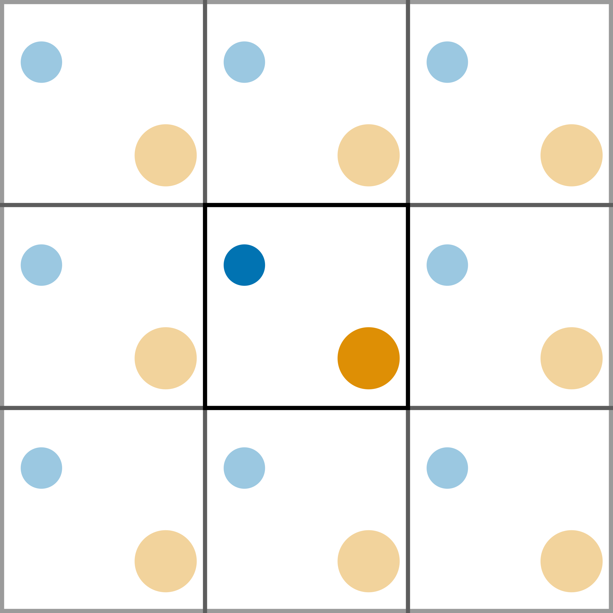
Figure 1. A two-dimensional example of a periodic cell.
When a particle reaches the cell wall it moves into the adjecent cell, and since all the cells are identical, it appears on the other side.
The code below modifies the update_pos and get_acceleration functions defined previously to account for the periodic boundary condition.
import numpy as np
import matplotlib.pyplot as plt
mass_of_argon = 39.948 # amu

def update_pos(x, v, a, dt, box_length):
    """
    Update the particle positions accounting for the
    periodic boundary condition.

    Parameters
    ----------
    x: ndarray of floats
        The positions of the particles in a single dimension
    v: ndarray of floats
        The velocities of the particles in a single dimension
    a: ndarray of floats
        The accelerations of the particles in a single dimension
    dt: float
        The timestep length
    box_length: float
        The size of the periodic cell

    Returns
    -------
    ndarray of floats:
        New positions of the particles in a single dimension
    """
    new_pos = x + v * dt + 0.5 * a * dt * dt
    #print(new_pos)
    new_pos = new_pos % box_length
    #print(new_pos)
    return new_pos

def lj_force(r, epsilon, sigma):
    """
    Implementation of the Lennard-Jones potential
    to calculate the force of the interaction.

    Parameters
    ----------
    r: float
        Distance between two particles (Å)
    epsilon: float
        Potential energy at the equilibrium bond
        length (eV)
    sigma: float
        Distance at which the potential energy is
        zero (Å)

    Returns
    -------
    float
        Force of the van der Waals interaction (eV/Å)
    """
    return 48 * epsilon * np.power(
        sigma / r, 13) - 24 * epsilon * np.power(
        sigma / r, 7)

def get_accelerations(positions, box_length, cutoff):
    """
    Calculate the acceleration on each particle as a
    result of each other particle.

    Parameters
    ----------
    positions: ndarray of floats
        The positions, in a single dimension, for all
        of the particles
    box_length: float
        The size of the periodic cell
    cutoff: float
        The distance after which the interaction
        is ignored

    Returns
    -------
    ndarray of floats
        The acceleration on each particle
    """
    accel_x = np.zeros((positions.size, positions.size))
    for i in range(0, positions.size - 1):
        for j in range(i + 1, positions.size):
            r_x = positions[j] - positions[i]
            r_x = r_x % box_length
            rmag = np.sqrt(r_x * r_x)
            force_scalar = lj_force(rmag, 0.0103, 3.4)
            force_x = force_scalar * r_x / rmag
            accel_x[i, j] = force_x / mass_of_argon
            accel_x[j, i] = - force_x / mass_of_argon
    return np.sum(accel_x, axis=0)
This means that we can use these new functions in our molecular dynamics simulation built previously.
from scipy.constants import Boltzmann
def update_velo(v, a, a1, dt):
"""
Update the particle velocities.
Parameters
----------
v: ndarray of floats
The velocities of the particles in a single dimension
a: ndarray of floats
The accelerations of the particles in a single dimension
at the previous timestep
a1: ndarray of floats
The accelerations of the particles in a single dimension
at the current timestep
dt: float
The timestep length
Returns
-------
ndarray of floats:
New velocities of the particles in a single dimension
"""
return v + 0.5 * (a + a1) * dt
def init_velocity(T, number_of_particles):
"""
Initialise the velocities for a series of particles.
Parameters
----------
T: float
Temperature of the system at initialisation
number_of_particles: int
Number of particles in the system
Returns
-------
ndarray of floats
Initial velocities for a series of particles
"""
R = np.random.rand(number_of_particles) - 0.5
return R * np.sqrt((Boltzmann / 1.602e-19) * T / mass_of_argon)
def run_md(dt, number_of_steps, initial_temp, x, box_length):
"""
Run a MD simulation.
Parameters
----------
dt: float
The timestep length
number_of_steps: int
Number of iterations in the simulation
initial_temp: float
Temperature of the system at initialisation
x: ndarray of floats
The initial positions of the particles in a single dimension
Returns
-------
ndarray of floats
The positions for all of the particles throughout the simulation
"""
cutoff = box_length / 2.
positions = np.zeros((number_of_steps, x.size))
v = init_velocity(initial_temp, x.size)
a = get_accelerations(x, box_length, cutoff)
for i in range(number_of_steps):
#print(i)
x = update_pos(x, v, a, dt, box_length)
a1 = get_accelerations(x, box_length, cutoff)
v = update_velo(v, a, a1, dt)
a = np.array(a1)
positions[i, :] = x
return positions
box_length = 10
x = np.array([0, 5, 9])
sim_pos = run_md(1e-1, 10000, 300, x, box_length)
%matplotlib inline
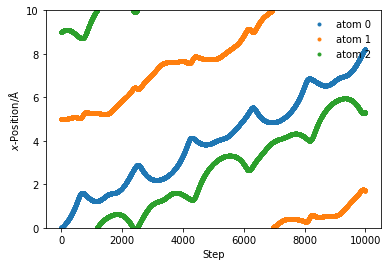
for i in range(sim_pos.shape[1]):
plt.plot(sim_pos[:, i], '.', label='atom {}'.format(i))
plt.ylim(0, box_length)
plt.xlabel(r'Step')
plt.ylabel(r'$x$-Position/Å')
plt.legend(frameon=False)
plt.show()
References
- Gumbart, J.; Trabuco, L. G.; Schreiner, E.; Villa, E.; Schulten, K. Structure 2009, 17 (11), 1453–1464. 10.1016/j.str.2009.09.010.