Build an MD simulation
We can now build our own one-dimensional molecular dynamics simulation. The Python code contains everything we need to build the MD simulation. Read though it (much of it has been discussed previously) and try to understand the flow of the code before running it to see what happens.
import numpy as np
import matplotlib.pyplot as plt
from scipy.constants import Boltzmann
mass_of_argon = 39.948 # amu

def lj_force(r, epsilon, sigma):
    """
    Implementation of the Lennard-Jones potential
    to calculate the force of the interaction.

    Parameters
    ----------
    r: float
        Distance between two particles (Å)
    epsilon: float
        Potential energy at the equilibrium bond
        length (eV)
    sigma: float
        Distance at which the potential energy is
        zero (Å)

    Returns
    -------
    float
        Force of the van der Waals interaction (eV/Å)
    """
    return 48 * epsilon * np.power(
        sigma, 12) / np.power(
        r, 13) - 24 * epsilon * np.power(
        sigma, 6) / np.power(r, 7)

def init_velocity(T, number_of_particles):
    """
    Initialise the velocities for a series of
    particles.

    Parameters
    ----------
    T: float
        Temperature of the system at
        initialisation (K)
    number_of_particles: int
        Number of particles in the system

    Returns
    -------
    ndarray of floats
        Initial velocities for a series of
        particles (eVs/Åamu)
    """
    R = np.random.rand(number_of_particles) - 0.5
    return R * np.sqrt(Boltzmann * T / (
        mass_of_argon * 1.602e-19))

def get_accelerations(positions):
    """
    Calculate the acceleration on each particle
    as a  result of each other particle.
    N.B. We use the Python convention of
    numbering from 0.

    Parameters
    ----------
    positions: ndarray of floats
        The positions, in a single dimension,
        for all of the particles

    Returns
    -------
    ndarray of floats
        The acceleration on each
        particle (eV/Åamu)
    """
    accel_x = np.zeros((positions.size, positions.size))
    for i in range(0, positions.size - 1):
        for j in range(i + 1, positions.size):
            r_x = positions[j] - positions[i]
            rmag = np.sqrt(r_x * r_x)
            force_scalar = lj_force(rmag, 0.0103, 3.4)
            force_x = force_scalar * r_x / rmag
            accel_x[i, j] = force_x / mass_of_argon
            accel_x[j, i] = - force_x / mass_of_argon
    return np.sum(accel_x, axis=0)

def update_pos(x, v, a, dt):
    """
    Update the particle positions.

    Parameters
    ----------
    x: ndarray of floats
        The positions of the particles in a
        single dimension
    v: ndarray of floats
        The velocities of the particles in a
        single dimension
    a: ndarray of floats
        The accelerations of the particles in a
        single dimension
    dt: float
        The timestep length

    Returns
    -------
    ndarray of floats:
        New positions of the particles in a single
        dimension
    """
    return x + v * dt + 0.5 * a * dt * dt

def update_velo(v, a, a1, dt):
    """
    Update the particle velocities.

    Parameters
    ----------
    v: ndarray of floats
        The velocities of the particles in a
        single dimension (eVs/Åamu)
    a: ndarray of floats
        The accelerations of the particles in a
        single dimension at the previous
        timestep (eV/Åamu)
    a1: ndarray of floats
        The accelerations of the particles in a
        single dimension at the current
        timestep (eV/Åamu)
    dt: float
        The timestep length

    Returns
    -------
    ndarray of floats:
        New velocities of the particles in a
        single dimension (eVs/Åamu)
    """
    return v + 0.5 * (a + a1) * dt

def run_md(dt, number_of_steps, initial_temp, x):
    """
    Run a MD simulation.

    Parameters
    ----------
    dt: float
        The timestep length (s)
    number_of_steps: int
        Number of iterations in the simulation
    initial_temp: float
        Temperature of the system at
        initialisation (K)
    x: ndarray of floats
        The initial positions of the particles in a
        single dimension (Å)

    Returns
    -------
    ndarray of floats
        The positions for all of the particles
        throughout the simulation (Å)
    """
    positions = np.zeros((number_of_steps, 3))
    v = init_velocity(initial_temp, 3)
    a = get_accelerations(x)
    for i in range(number_of_steps):
        x = update_pos(x, v, a, dt)
        a1 = get_accelerations(x)
        v = update_velo(v, a, a1, dt)
        a = np.array(a1)
        positions[i, :] = x
    return positions

x = np.array([1, 5, 10])
sim_pos = run_md(0.1, 10000, 300, x)

%matplotlib inline
for i in range(sim_pos.shape[1]):
    plt.plot(sim_pos[:, i], '.', label='atom {}'.format(i))
plt.xlabel(r'Step')
plt.ylabel(r'$x$-Position/Å')
plt.legend(frameon=False)
plt.show()
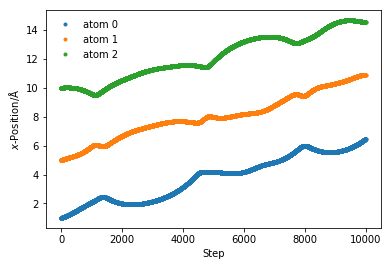
We can see how the particles interact with each other separated by about the minimum of the LJ and moving in tandem through the system.
It is possible to run the simulation at a series of different initial starting positions by varying values in the array x.