Solutions#
It’s time to plot.
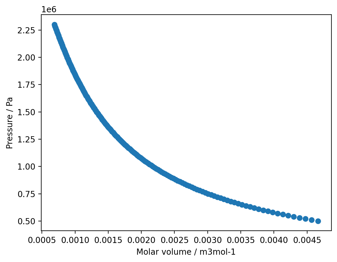
1. You have been provided with an experimental pressure/volume isotherm for SF\(_{6}\) at \(298\,\)K in the form of a csv file.
a) Read in the experimental data using numpy, convert to SI units and plot the isotherm using matplotlib.
import matplotlib.pyplot as plt
import numpy as np

p, v = np.loadtxt('isotherm.csv', unpack=True, delimiter=',')

p *= 10 ** 5 # Convert from bar to Pa
v /= 10 ** 3 # Convert from Lmol-1 to m3mol-1

plt.plot(v, p, 'o')
plt.xlabel('Molar volume / m3mol-1')
plt.ylabel('Pressure / Pa')

plt.show()
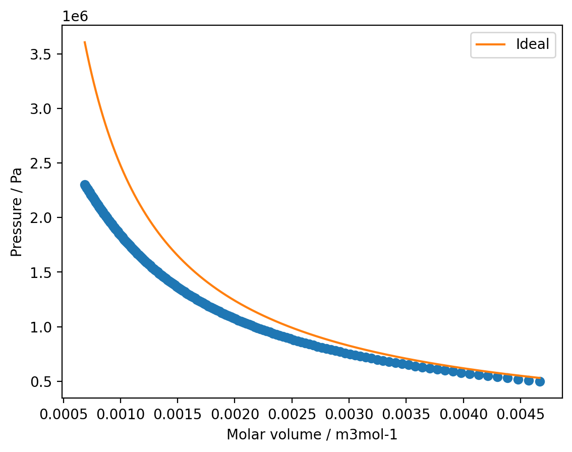
b) Assuming ideality, the isotherm should be well modelled by the ideal gas law:
where \(p\) is the pressure, \(v\) is the molar volume (\(V / n\)), \(R\) is the gas constant and \(T\) is the temperature.
Write a function to calculate the pressure with the ideal gas law and use this to model the SF\(_{6}\) isotherm between \(v = 6.87 \times 10^{-4}\,\)m\(^{3}\,\)mol\(^{-1}\) and \(v = 4.47 \times 10^{-3}\,\)m\(^{3}\,\)mol\(^{-1}\). Plot your modelled isotherm against the experimental data.
import scipy

def ideal_pressure(v, T):
    """
    Calculate the pressure of an ideal gas for a range of molar volumes.

    Args:
        v (np.ndarray): A numpy array containing the molar volumes for which to evaluate the pressure.
        T (float): The temperature.

    Returns:
        (np.ndarray): A numpy array of the evaluated pressures.
    """

    return scipy.constants.R * T / v

temperature = 298
v_model = np.linspace(min(v), max(v), 1000)

p_ideal = ideal_pressure(v_model, temperature)

plt.plot(v, p, 'o')
plt.plot(v_model, p_ideal, label='Ideal')
plt.xlabel('Molar volume / m3mol-1')
plt.ylabel('Pressure / Pa')

plt.legend()
plt.show()
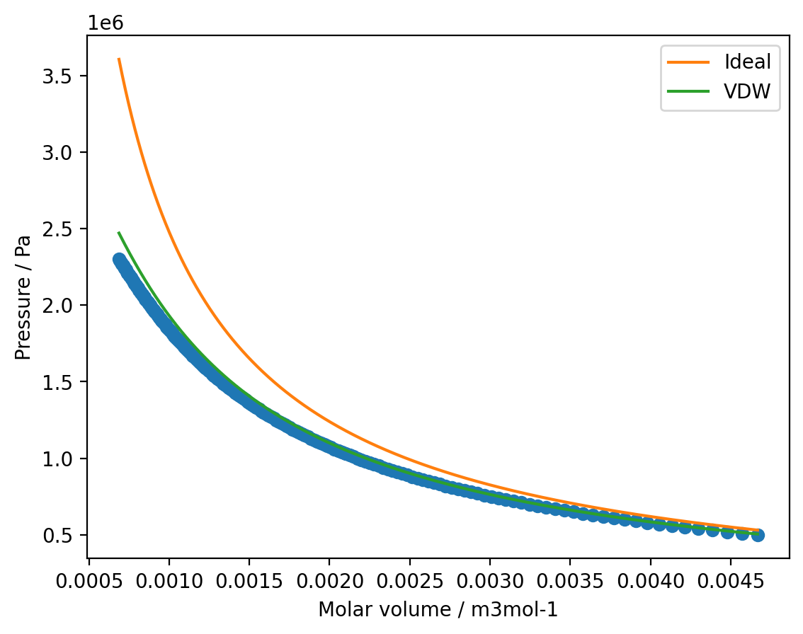
c) Non-ideality due to intermolecular interactions and other factors can be accounted for (in part) by the Van der Waals equation of state:
where \(p\) is the pressure, \(R\) is the gas constant, \(v\) is the molar volume and \(a\) and \(b\) are system dependent constants that describe the strength of the interactions and excluded volume effects respectively.
Write a function to calculate the pressure with the Van der Waals equation and use this to model the SF\(_{6}\) isotherm with \(a = 7.857 \times 10^{-1}\,\)m\(^{6}\,\)Pa\(\,\)mol\(^{-2}\) and \(b = 8.79 \times 10^{-5}\,\)m\(^{3}\,\)mol\(^{-1}\) between \(v = 6.87 \times 10^{-4}\,\)m\(^{3}\,\)mol\(^{-1}\) and \(v = 4.47 \times 10^{-3}\,\)m\(^{3}\,\)mol\(^{-1}\). Plot your modelled isotherm and compare this against the idealised curve and the experimental data.
def vdw_pressure(v, T, a, b):
    """
    Calculate the pressure according to the Van der Waals equation for a range of molar volumes.

    Args:
        v (np.ndarray): A numpy array containing the molar volumes for which to evaluate the pressure.
        T (float): The temperature.
        a (float): A system-dependent constant that represents the strength of the intermolecular interactions.
        b (float): A system-dependent constant that accounts for the volume excluded by the finite size of the molecules.

    Returns:
        (np.ndarray): A numpy array of the evaluated pressures.
    """

    return (scipy.constants.R * T) / (v - b) - a / v ** 2

a = 7.857e-01
b = 8.79e-05

p_vdw = vdw_pressure(v_model, temperature, a, b)

plt.plot(v, p, 'o')
plt.plot(v_model, p_ideal, label='Ideal')
plt.plot(v_model, p_vdw, label='VDW')
plt.xlabel('Molar volume / m3mol-1')
plt.ylabel('Pressure / Pa')

plt.legend()
plt.show()
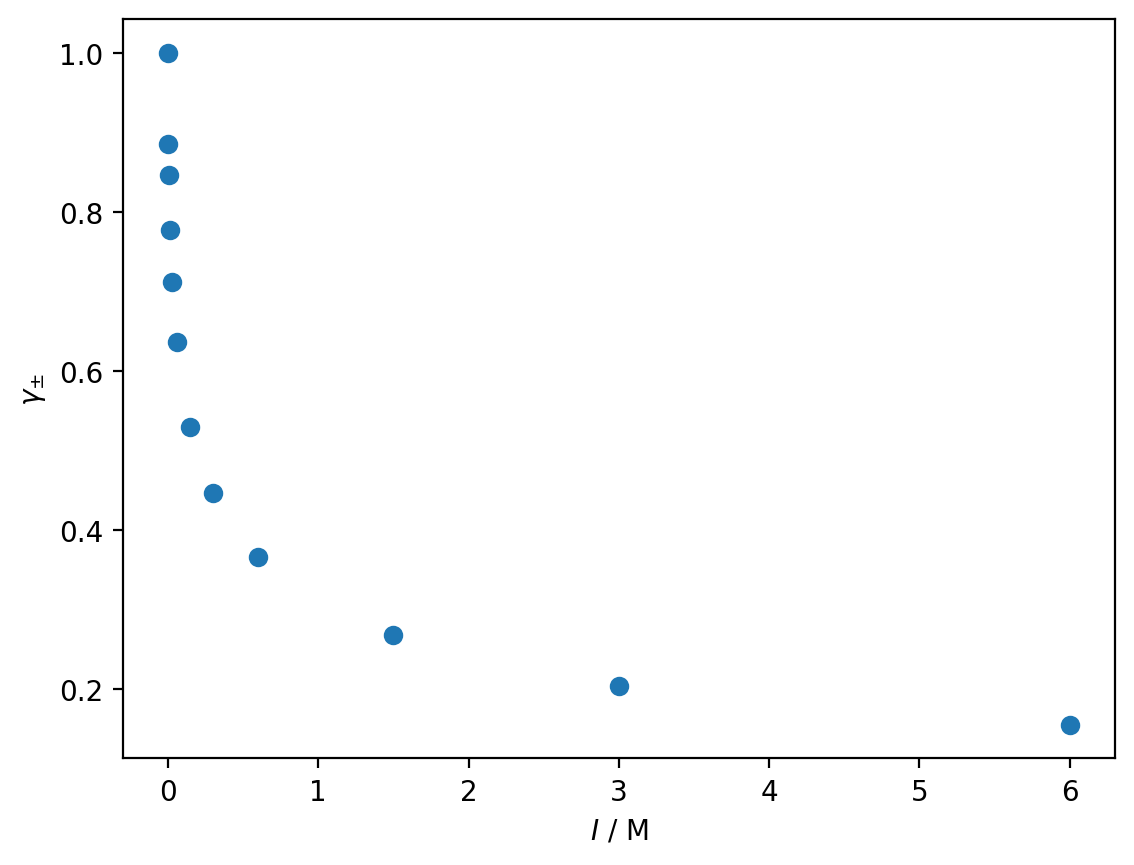
2. The mean activity of ions in solution can be measured experimentally. You have been provided with the mean activity of Na\(_{2}\)SO\(_{4}\) at \(298\,\)K for a range of ionic strengths: activity.dat
a) Use matplotlib to render a scatter plot of the mean activity as a function of the ionic strength \(I\).
ionic_strength, mean_activity = np.loadtxt('activity.dat', unpack=True)

plt.plot(ionic_strength, mean_activity, 'o')
plt.xlabel('$I$ / M')
plt.ylabel(r'$\gamma_{\pm}$')

plt.show()
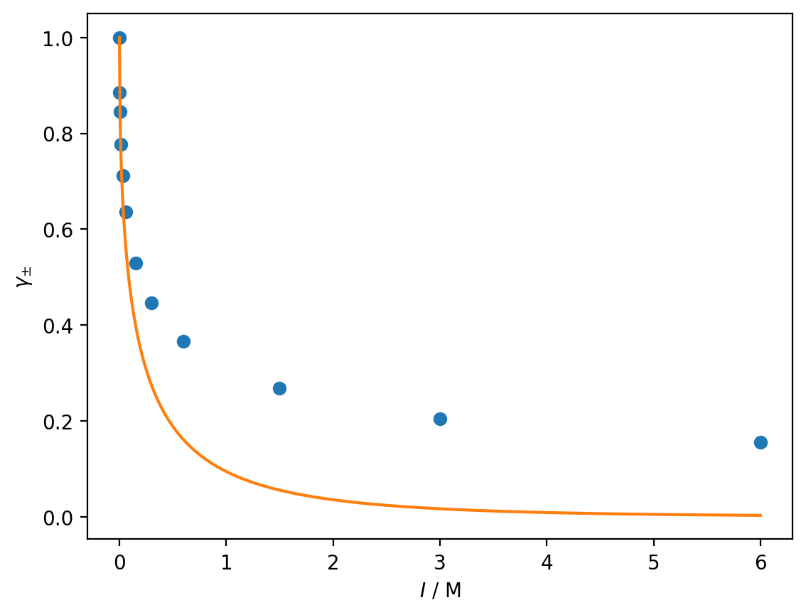
b) The mean activity can be predicted by the Debye-Huckel limiting law:
where \(z_{+}\) and \(z_{-}\) are the charges of the cations and anions, \(I\) is the ionic strength and \(A\) is a solvent and temperature dependent constant.
Write a function to calculate the mean activity according to the Debye-Huckel limiting law (feel free to reuse your code from previous exercises). Using \(A = 1.179\,\)M\(^{\frac{1}{2}}\), plot the Debye-Huckel mean activity from \(I = 0\,\)M to \(I = 6\,\)M and compare this with the experimental values.
def debye_huckel(I, z_plus, z_minus, A):
    return np.exp(-abs(z_plus * z_minus) * A * np.sqrt(I))

I_dh = np.linspace(0, 6, 1000)
gamma_dh = debye_huckel(I_dh, 1, -2, 1.179)

plt.plot(ionic_strength, mean_activity, 'o')
plt.plot(I_dh, gamma_dh)
plt.xlabel('$I$ / M')
plt.ylabel(r'$\gamma_{\pm}$')

plt.show()
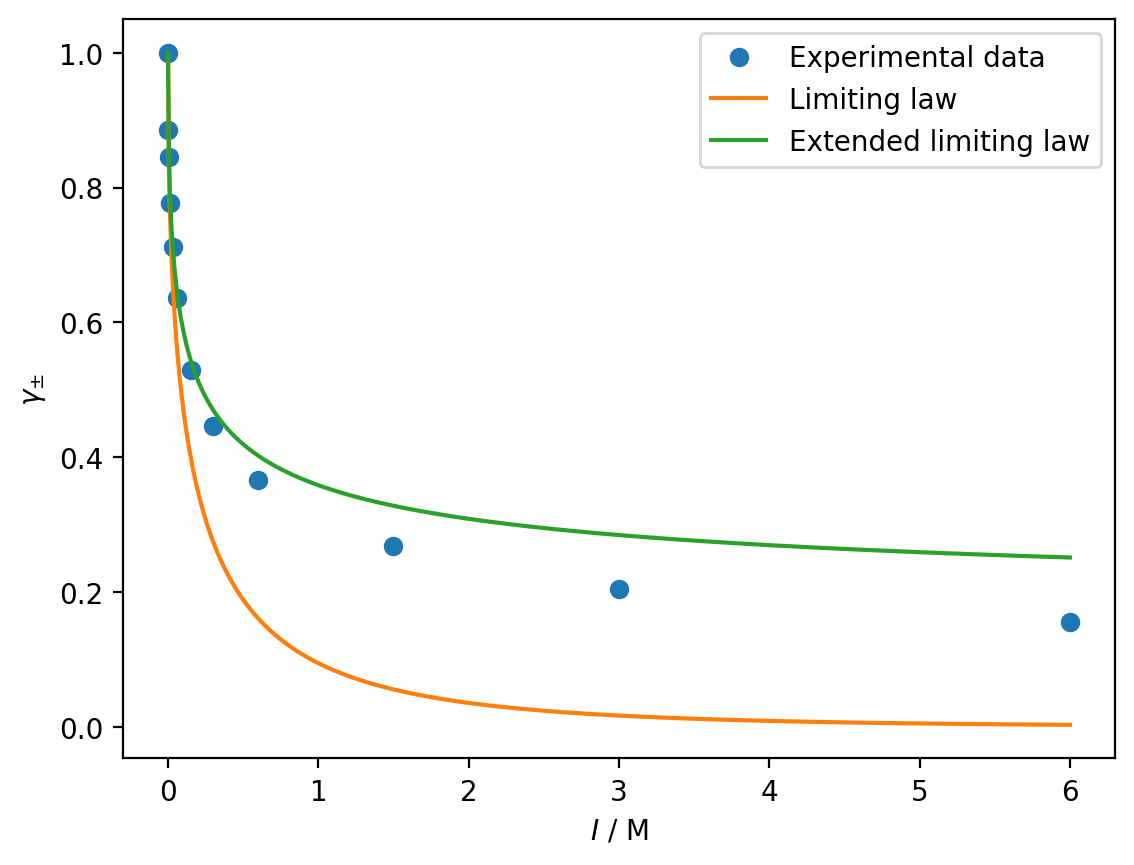
c) There are several extensions of the Debye-Huckel limiting law that aim to improve its description of the mean activity outside of the dilute limit. One such extension is:
where \(B\) is another solvent and temperature dependent constant and \(a_{0}\) is the distance of closest approach (expected to be proportional to the closest distance between ions in solution).
Write a function to calculate the mean activity according to the extended Debye-Huckel limiting law. Using \(B = 18.3\) and \(a_{0} = 0.071\), plot the extended Debye-Huckel mean activity from \(I = 0\,\)M to \(I = 6\,\)M and compare this with the experimental values and the original Debye-Huckel limiting law.
def debye_huckel_extended(I, z_plus, z_minus, A, B, a_0):
    return np.exp(-abs(z_plus * z_minus) * ((A * np.sqrt(I)) / (1 + B * a_0 * np.sqrt(I))))

gamma_dhe = debye_huckel_extended(I_dh, 1, 2, 1.179, 18.3, 0.071)

plt.plot(ionic_strength, mean_activity, 'o', label='Experimental data')
plt.plot(I_dh, gamma_dh, label='Limiting law')
plt.plot(I_dh, gamma_dhe, label='Extended limiting law')
plt.xlabel('$I$ / M')
plt.ylabel(r'$\gamma_{\pm}$')

plt.legend()
plt.show()