Minimisation#
As we have touched on already, the curve_fit function uses least-squares regression to fit models to datasets. Mathematically, this corresponds to the following process:
where each \(y_{i}\) is an experimental \(y\)-value and each \(f_{\theta}(x_{i})\) is our model’s prediction for that \(y\)-value for a given set of model parameters \(\theta\). To clarify what we mean by “model parameters”, in the context of a linear model, these would be the slope \(m\) and the intercept \(c\), whereas for a quadratic model, these would be \(a\), \(b\) and \(c\) as per the standard form of a quadratic equation.
So, what curve_fit is really doing under the hood is minimising \([y_{i} - f_{\theta}(x_{i})]^{2}\) with respect to \(\theta\). Hopefully you can see where the term “least-squares” comes from: we are minimising the sum of squared differences between the experimental data and our model’s predictions. When we provide information about the variance of individual data points via the sigma argument, we move from ordinary least-squares to weighted least-squares:
where each \(\sigma_{i}\) is the variance associated with a given \(y\)-value. By dividing by the variance of each data point, we effectively weight our final model to stick closer to the data points with lower variance.
The brief explanation above is present for two reasons. Firstly, it is there simply to explain how the curve_fit function actually works, so that it seems like less of a “black box”. Secondly, it showcases quite nicely the power of function minimisation. When performing least-squares regression, we are minimising a sum of squared differences (sometimes called \(\chi^{2}\)), a function which calculates the error between a model’s predictions and some dataset. This is one very useful example in the context of data analysis, but there are many more situations besides this in which we can solve problems by minimising the value of a given function.
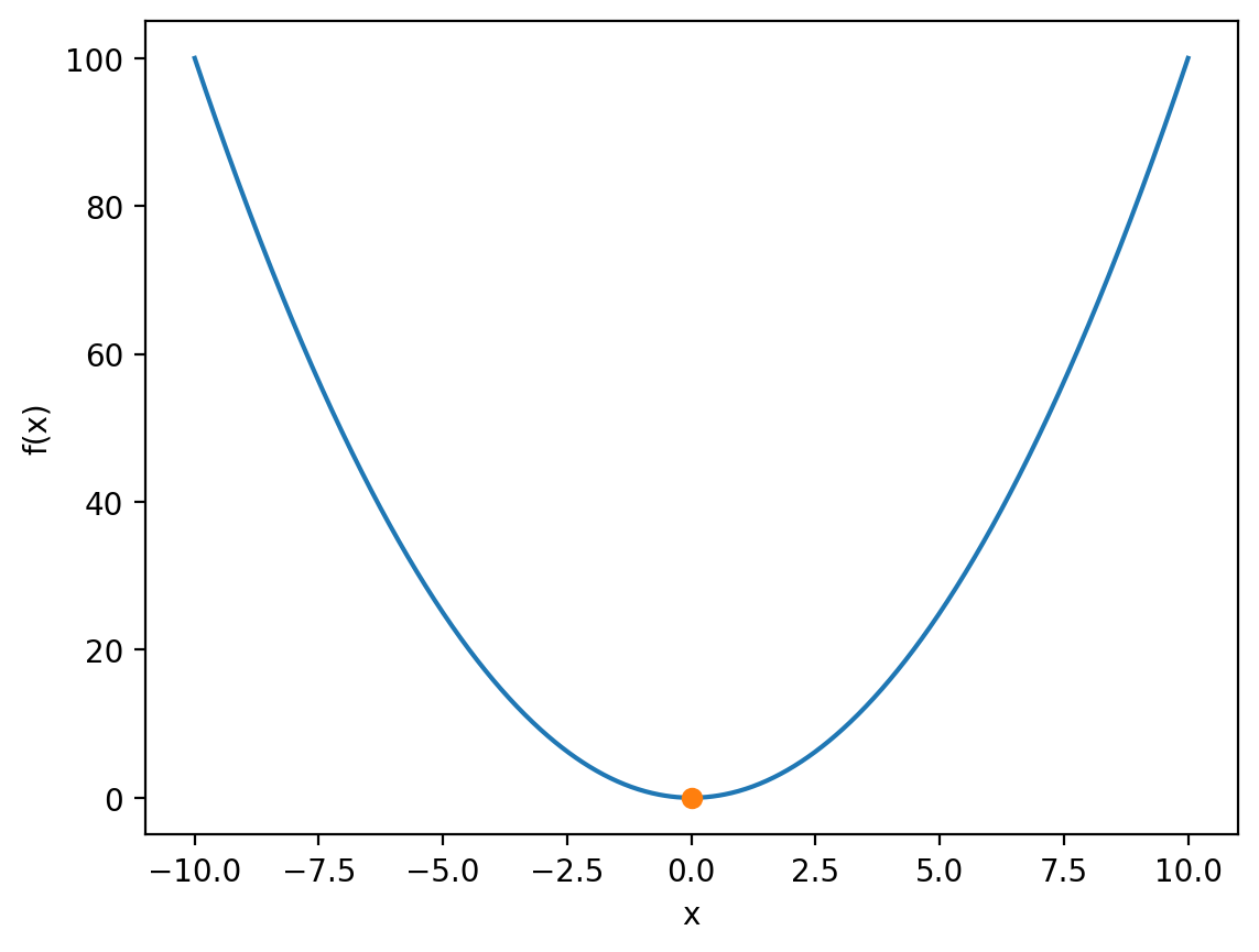
For an abstract example, consider the function:
import matplotlib.pyplot as plt
import numpy as np

x = np.linspace(-10, 10, 1000)
f_x = x ** 2

plt.plot(x, f_x)
plt.xlabel('x')
plt.ylabel('f(x)')

plt.show()

Now obviously as human beings, we can find the minimum of this function analytically via calculus, but what if we wanted to minimise \(f(x)\) numerically?
We can perform numerical minimisation with the minimize function, again from the scipy library:
from scipy.optimize import minimize
Similar to curve_fit, optimize requires us to define the function that we would like to minimise:
def x_squared(x):
    """Calculate f(x) = x^2 for a range of x-values.

    Args:
        x (np.ndarray): The x-values.

    Returns:
        np.ndarray: The value of f(x) for each input x.

    """

    return x ** 2
Now we can call the minimize function:
minimize(x_squared, x0=[5])
  message: Optimization terminated successfully.
  success: True
   status: 0
      fun: 6.914540092077327e-16
        x: [-2.630e-08]
      nit: 3
      jac: [-3.769e-08]
 hess_inv: [[ 5.000e-01]]
     nfev: 8
     njev: 4
Notice that we supplied minimize with two arguments: the name of the function that we would like to minimize x_squared and a list [5]. The second argument x0 is our initial guess for the minimum. Now again, this is a somewhat trivial example, we know that the minimum is at \(0\), but here we set our initial guess to \(5\) to show that minimize can get to the correct result on its own. The reason that this argument is a list rather than a float is that the minimize function can minimise functions with respect to multiple variables simultaneously e.g. the set of parameters \(\theta\) in least-squares regression (in which case you would need an initial guess for each of those variables).
As you can see above, the minimize function provides us with a lot of information. For now, we only really care about the x row, which contains the value of \(x\) which minimises \(f(x)\):
minimisation_data = minimize(x_squared, x0=[5])
x_min = minimisation_data.x[0] # Indexing used as minimize will return a numpy array even if there is only one variable being minimised).

print(f'arg min f(x) = {x_min} (very nearly 0)')
arg min f(x) = -2.6295513100293988e-08 (very nearly 0)
We can visualise the minimum by plotting it on top of our original curve:
f_at_x_min = x_squared(x_min) # Get f(x) at x = x_min

plt.plot(x, f_x)
plt.plot(x_min, f_at_x_min, 'o')
plt.xlabel('x')
plt.ylabel('f(x)')

plt.show()
Local minima#
Minimising \(x^{2}\) is not the most difficult task, both because it can be done analytically, and because it has a single global minimum. In other words, \(x^{2}\) is at its lowest value at \(x = 0\) and grows monotonically everywhere else from \(-\infty\) to \(\infty\). Most functions are, in this sense, not so friendly.
For example, consider the function:
def oscillatory_quadratic(x):
    """Calculates f(x) = x^2 - 10 cos 2pi x + 10 for a range of x-values.

    Args:
        x (np.ndarray): The x-values.

    Returns:
        np.ndarray: The value of f(x) for each input x.

    """
    return x ** 2 - 10 * np.cos(2 * np.pi * x) + 10

x = np.linspace(-2 * np.pi, 2 * np.pi, 1000)
f_x = oscillatory_quadratic(x)

plt.plot(x, f_x)
plt.xlabel('x')
plt.ylabel('f(x)')

plt.show()
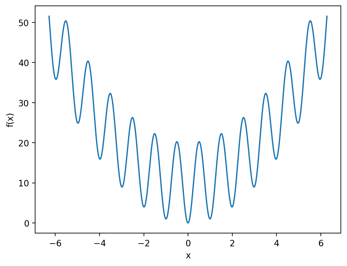
Again it’s easy enough for us to see that the minimum is at \(x = 0\), but let’s try to compute this numerically.
minimisation_data = minimize(oscillatory_quadratic, x0=[5.25])
min_x = minimisation_data.x[0]

print(f'arg min f(x) = {min_x}')
arg min f(x) = -0.9949586450236011
Oh dear, this time we’re not getting \(x = 0\).
initial_guess = 5.25
# get f(x) at the initial guess and at x_min
init_f_x = oscillatory_quadratic(initial_guess)
f_x_at_min = oscillatory_quadratic(min_x)

plt.plot(x, f_x)
plt.plot(min_x, f_x_at_min, 'o', label='Local minimum')
plt.plot(initial_guess, init_f_x, 'o', label='Initial guess')
plt.xlabel('x')
plt.ylabel('f(x)')

plt.legend()
plt.show()
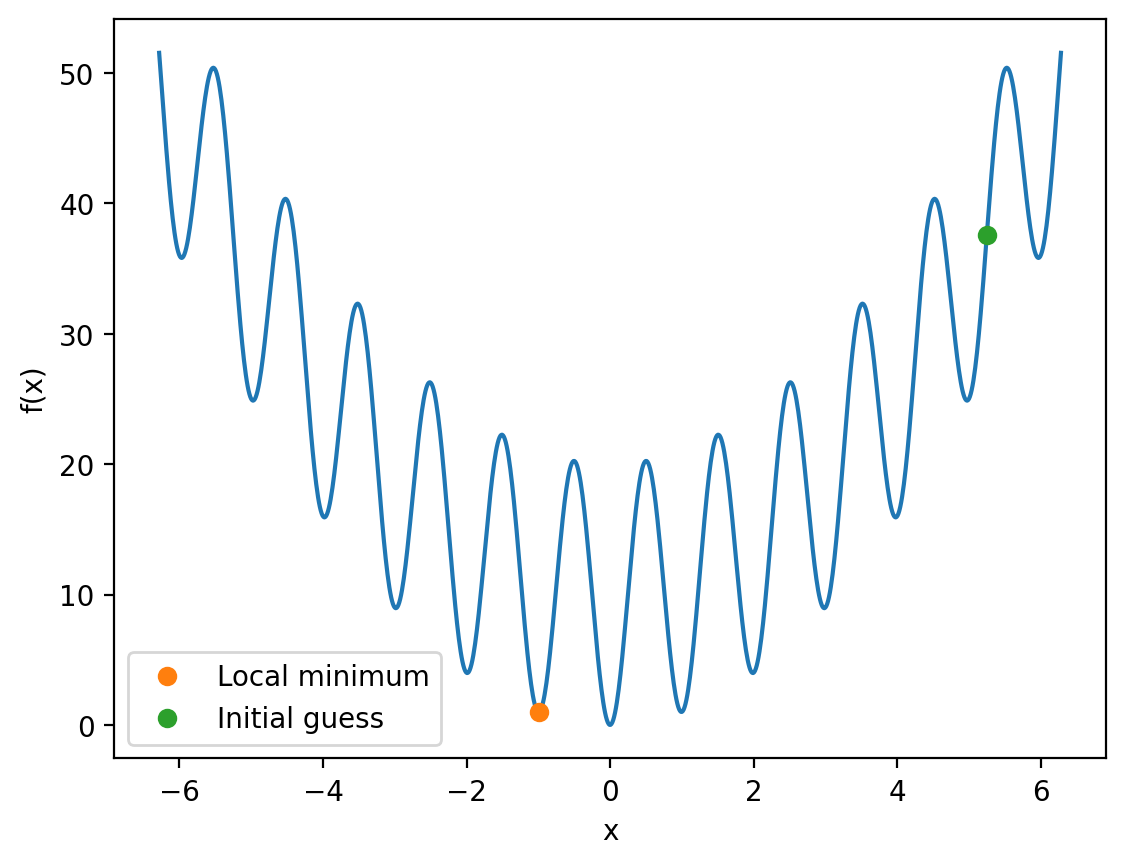
As you can see, the minimize function has located a local minimum at \(x \approx -1\), but has failed to reach the global minimum at \(x = 0\).
This example highlights nicely that using the minimize function - and more generally the process of function optimisation - is not always as straightforward as our \(x^{2}\) example. Let’s take a second to think about why we might get stuck in a local minimum. If we were to find the minimum analytically, we would differentiate \(f(x)\) and set the derivative to zero:
To us human beings, it is clear that the equation above is only true when \(x = 0\), as the first term \(2x\) will be non-zero everywhere else. From the perspective of the minimize function however, the gradient gets much closer to zero for all integers \(n\) if \(x = \pi n\) (as the second term of the derivative will be \(0\)). This is why numerical methods for function minimisation get stuck in local minima: by definition the gradient at these points is small or even zero, hence they look (mathematically) just like the global minimum.
So, how can we solve this problem? Well, for one thing, we can change our initial guess:
minimisation_data = minimize(oscillatory_quadratic, x0=[1.25])
min_x = minimisation_data.x[0]

print(f'arg min f(x) = {min_x}')
arg min f(x) = -6.982386725092019e-09
By moving our initial guess closer to where we expect the global minimum to be, we recover the correct result:
initial_guess = 1.25
init_f_x = oscillatory_quadratic(initial_guess)
f_x_at_min = oscillatory_quadratic(min_x)

plt.plot(x, f_x)
plt.plot(min_x, f_x_at_min, 'o', label='Global minimum')
plt.plot(initial_guess, init_f_x, 'o', label='Initial guess')
plt.xlabel('x')
plt.ylabel('f(x)')

plt.legend()
plt.show()
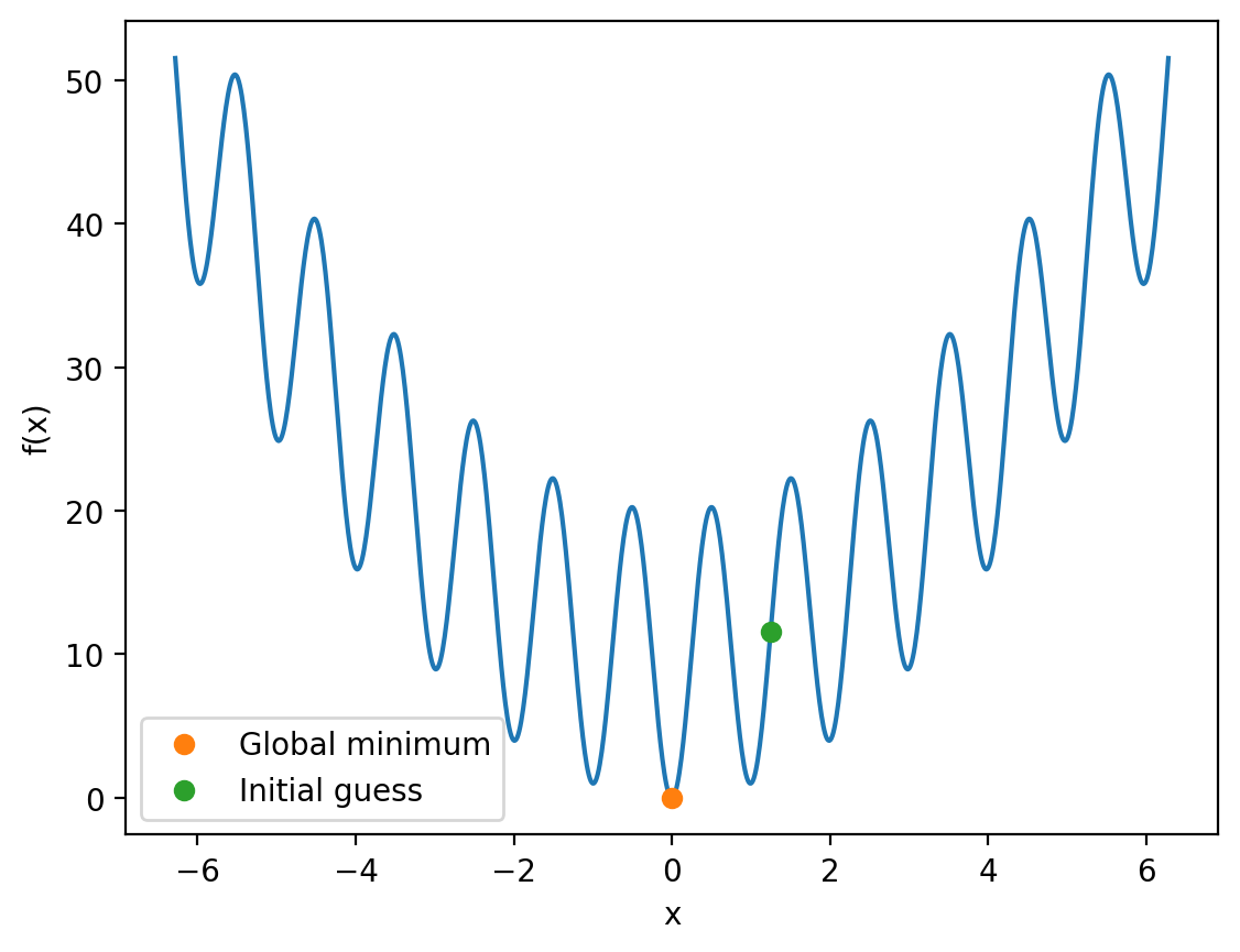
In this case, we were able to improve our initial guess because we knew where we expected the global minimum to be. This was possible due to the fact that we are dealing with a relatively simple one-dimensional function, but there is no guarantee in general that this will be possible.
The more general point here is that minimisation algorithms (such as those used by the minimize function) are not perfect and may well be sensitive to the initial guess. It is therefore prudent to think about what we know about the function that we are trying to minimise in order to select a sensible initial guess. For a trivial example, if we know that our function goes to \(\infty\) for all \(x > 5\), then we would obviously want our initial guess to be \(< 5\).