Linear regression#
We have now built up all of the knowledge necessary to do some data analysis. We’re going to start with something that you’re probably very familiar with: finding a line of best fit.
In all of the following examples, we will be dealing with abstract data (i.e. \(x\) and \(y\) rather than volume and pressure or time and concentration etc), so as to focus on the methodology behind what we are doing rather than the details of the data itself. There will be frequent references to various statistical concepts, but don’t stress too much if you are unfamiliar with any of the terminology: this is not a stats course.
Let’s imagine that we’ve been given some experimental data that is evidently linear:
import matplotlib.pyplot as plt
import numpy as np

x, y = np.loadtxt('linear.csv', delimiter=',', unpack=True)

plt.plot(x, y, 'o')
plt.xlabel('x')
plt.ylabel('y')

plt.show()
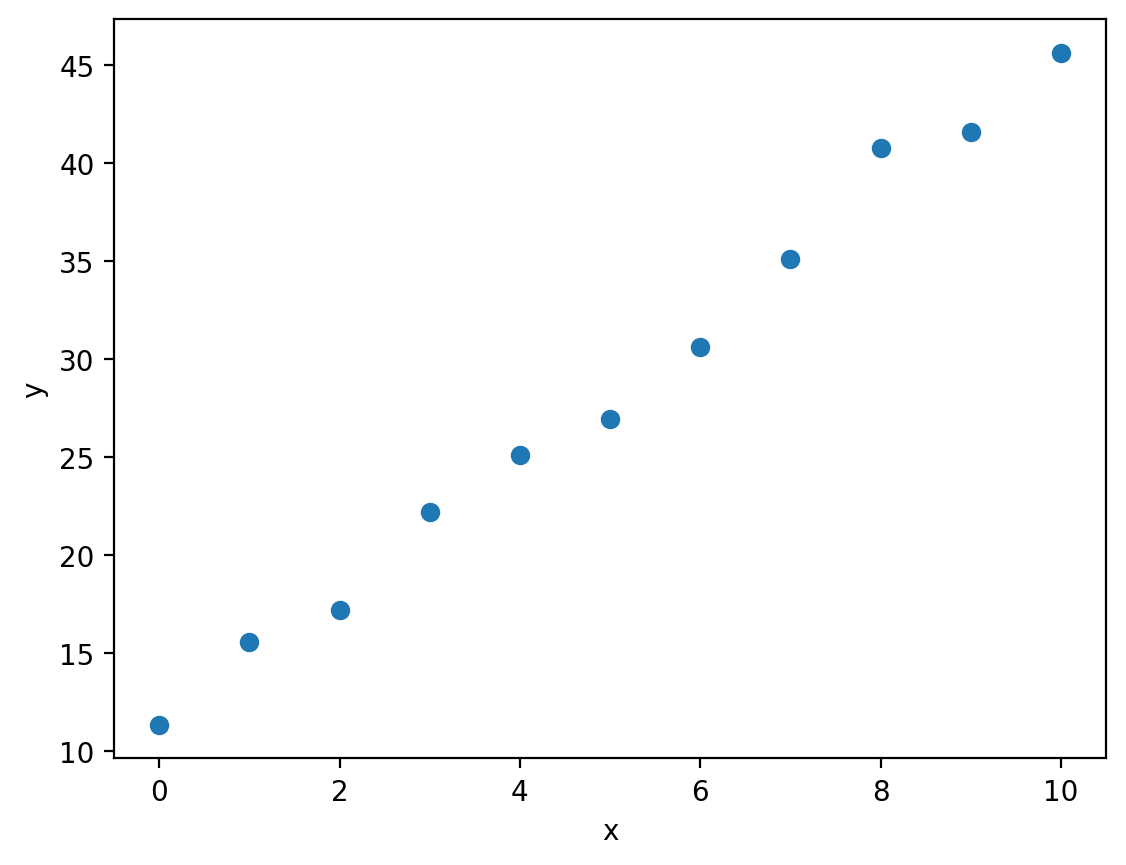
You can download linear.csv here.
In order to find a line of best fit, we would like to do linear regression. In short, we want to find the line:
(where \(m\) is the slope and \(c\) is the intercept), that is as close as possible to all the experimental data points. There are many ways to do linear regression in Python, but perhaps the simplest is the linregress function from the scipy library:
from scipy.stats import linregress

regression_data = linregress(x, y)

print(regression_data)
LinregressResult(slope=np.float64(3.434454545454545), intercept=np.float64(11.204090909090908), rvalue=np.float64(0.9961041753472445), pvalue=np.float64(8.369268779950266e-11), stderr=np.float64(0.10134983826003473), intercept_stderr=np.float64(0.5995937291506074))
The first thing you might notice about the code above is that the import statement looks a little different to those we have seen before. The from keyword allows to import individual functions or constants from a package rather than the whole thing. In this example, we have imported just the linregress function, which means we can call that function by typing linregress(x, y) rather than running import scipy and then having to type out scipy.stats.linregress(x, y). To further clarify this, you may recall that we have made frequent use of scipy to access important physical constants such as \(h\) and \(k_{\mathrm{B}}\) by typing scipy.constants.h or scipy.constants.k. Using the from keyword, we could instead type:
from scipy.constants import h, k

print(h, k)
6.62607015e-34 1.380649e-23
Coming back to the rest of our linear regression code, we called the linregress functions with two arguments: x and y:
regression_data = linregress(x, y)
These variables contain the experimental \(x\) and \(y\)-data as plotted previously. We stored the output of the linregress function in a variable called regression_data and then passed this to the print function:
print(regression_data)
The information returned from the linregress function contains the slope \(m\) and the intercept \(c\) of the line of best fit, alongside other useful information which we will discuss further shortly.
regression_data
LinregressResult(slope=np.float64(3.434454545454545), intercept=np.float64(11.204090909090908), rvalue=np.float64(0.9961041753472445), pvalue=np.float64(8.369268779950266e-11), stderr=np.float64(0.10134983826003473), intercept_stderr=np.float64(0.5995937291506074))
We can access the slope \(m\) and the intercept \(c\) as regression_data.slope and regression_data.intercept respectively:
print(f'm = {regression_data.slope}')
print(f'c = {regression_data.intercept}')
m = 3.434454545454545
c = 11.204090909090908
We now have all the information we need to construct and plot our line of best fit:
y_best_fit = regression_data.slope * x + regression_data.intercept # y = mx + c

plt.plot(x, y, 'o', label='Experimental data')
plt.plot(x, y_best_fit, label='Line of best fit')
plt.xlabel('x')
plt.ylabel('y')

plt.legend()
plt.show()
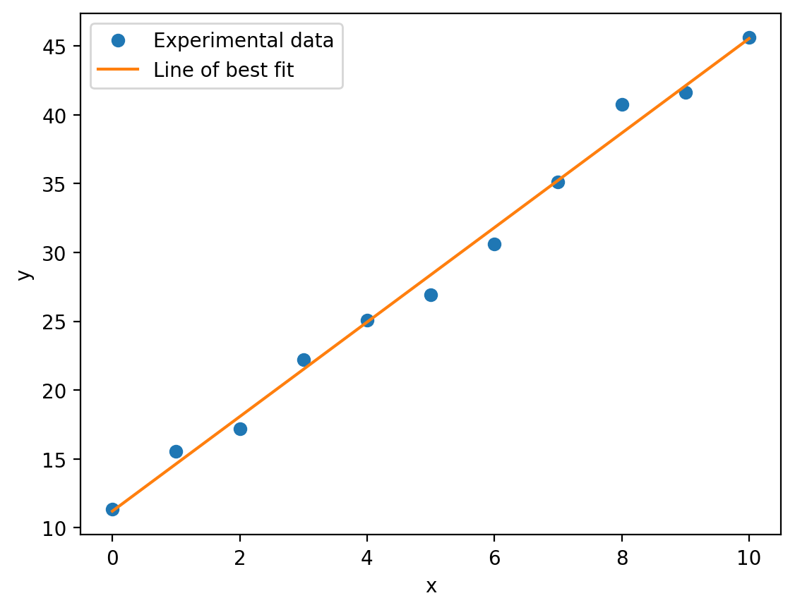
It’s worth emphasising at this stage that whilst the example is wholly abstract (\(x\) and \(y\) have no physical meaning and have no units), the same procedure could easily be applied to any linear dataset you might wish to analyse.
In addition to the slope and intercept of the line of best fit, the linregress function also gives us access to the standard error associated with both values via regression_data.stderr and regression_data.intercept_stderr:
print(f'm = {regression_data.slope} +/- {regression_data.stderr}')
print(f'c = {regression_data.intercept} +/- {regression_data.intercept_stderr}')
m = 3.434454545454545 +/- 0.10134983826003473
c = 11.204090909090908 +/- 0.5995937291506074
The linregress function uses the ordinary least-squares method to optimise \(m\) and \(c\), which assumes that the uncertainty (more specifically the variance) of all the experimental measurements are equal i.e. all the error bars are the same size. In the example we have worked through above, this assumption is valid (there are no error bars on our plot), but what if we want to account for data with some variance associated with each data point?
Accounting for uncertainties#
Let’s add some uncertainty to the experimental \(y\)-data from our previous example:
y_err = [1.55, 1.55, 1.53, 1.53, 1.33, 1.33, 1.33, 1.12, 1.02, 0.9, 0.9] # variance in each data point

plt.errorbar(x, y, y_err, fmt='o')
plt.xlabel('x')
plt.ylabel('y')

plt.show()
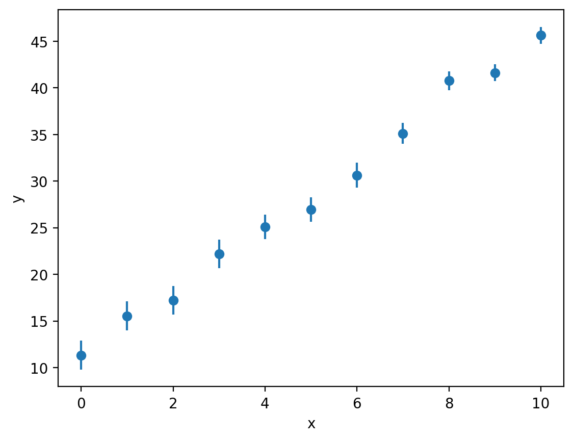
As you can see above, we can plot error bars using plt.errorbar, passing the size of each error bar as a third argument (here passed as the variable y_err). The fmt keyword argument is used to prevent matplotlib from joining each point with a line (this is roughly equivalent how we can pass strings such as 'o' or 'o-' to the plt.plot function to change how the data is rendered).
To perform linear regression on this dataset that explicitly accounts for the error bars, we are going to use the curve_fit function:
from scipy.optimize import curve_fit
Given that we’re trying to fit a straight line, you might be wondering why on earth we’re using a function called curve_fit. Simply put, curve_fit is a much more robust general-use function than linregress (it is not limited to linear regression) and it has a keyword argument sigma that can be used to explicitly account for uncertainties in the experimental \(y\)-data using the weighted least-squares method.
As mentioned above, curve_fit is not limited to fitting straight lines (hence the curve in the name). As a result, we have to specify the model we would like to try to fit to our dataset. In this case, our data is linear, so the model we are going to try and fit is the equation of a straight line:
where \(m\) is the slope and \(c\) is the intercept. We can define this model in Python as a function:
def straight_line(x, m, c):
    """Calculate y = mx + c (the equation of a straight line).

    Args:
        x (np.ndarray): A numpy array containing all of the x-values.
        m (float): The slope of the line.
        c (float): The y-intercept of the line.

    Returns:
        np.ndarray: The y-values.

    """

    return m * x + c
We can now pass our function as an argument to curve_fit, also passing the experimental \(x\) and \(y\) data as well as the uncertainties using the sigma keyword argument:
regression_data = curve_fit(straight_line, x, y, sigma=y_err)
curve_fit returns a tuple of two elements:
regression_data
(array([ 3.45325015, 11.13753085]),
 array([[ 0.01099572, -0.06900366],
        [-0.06900366,  0.53969832]]))
The first of these is a numpy array containing the optimised parameters for our model in the order they are specified in the function definition. In this case, our straight_line function takes the arguments x, m and c:
def straight_line(x, m, c):
m comes before c, so the same order will be reflected in the optimised parameters:
regression_data[0]
array([ 3.45325015, 11.13753085])
The second element of regression_data is the covariance matrix, again in the form of a numpy array:
regression_data[1]
array([[ 0.01099572, -0.06900366],
       [-0.06900366,  0.53969832]])
Without getting into the underlying statistics, the important data here is on the diagonal of this matrix. Again in the same order as specified in the function definition, each element on the diagonal is the variance associated with that parameter.
slope, intercept = regression_data[0]
covariance_matrix = regression_data[1]
slope_variance = covariance_matrix[0,0] # First element of the diagonal, row 1 column 1
intercept_variance = covariance_matrix[1,1] # Second element of the diagonal, row 2 column 2

print(f'm = {slope} +/- {np.sqrt(slope_variance)}')
print(f'c = {intercept} +/- {np.sqrt(intercept_variance)}')
m = 3.453250150061519 +/- 0.10486045758833921
c = 11.137530849160365 +/- 0.7346416256182807
Unlike when we used the linregress function, these errors actually account for the uncertainties in the experimental data. We take the square root here to get the standard error rather than the variance associated with each parameter. We can visualise our fitted model (our line of best fit) just like we did before:
y_model = straight_line(x, slope, intercept) # y = mx + c

plt.errorbar(x, y, y_err, fmt='o', label='Experimental data')
plt.plot(x, y_model, label='Line of best fit')
plt.xlabel('x')
plt.ylabel('y')

plt.legend()
plt.show()
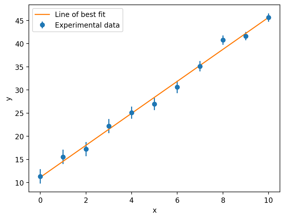
In this case, our final plot (and our values of \(m\) and \(c\)) are pretty similar whether we use the ordinary least-squares (linregress) or weighted least-squares (curve_fit with sigma) methods, but this is certainly not guaranteed to be the case and it is therefore very important to propagate experimental uncertanties through to our fitted model parameters when possible.