
In the previous tutorial, we were introduced to collections in the form of lists, tuples, and dictionaries. The python package NumPy provides a further example of a collection: an array. Arrays are collections which are engineered to easily and efficiently facilitate calculations.
For example, say we have conducted an experiment to determine the melting point of water. We have repeated this experiment 10 times to obtain a more accurate calculation of the melting point. The results from the experiment can be observed in the table below.
| Experiment | Melting Point ($^{\circ}$C) |
|---|---|
| 1 | 98.5 $\pm$ 0.1 |
| 2 | 99.9 $\pm$ 0.1 |
| 3 | 100.6 $\pm$ 0.1 |
| 4 | 99.3 $\pm$ 0.1 |
| 5 | 100.7 $\pm$ 0.1 |
| 6 | 99.4 $\pm$ 0.1 |
| 7 | 98.4 $\pm$ 0.1 |
| 8 | 99.5 $\pm$ 0.1 |
| 9 | 99.3 $\pm$ 0.1 |
| 10 | 100.7 $\pm$ 0.1 |
We want to store this information in a NumPy array so that we can calculate certain properties. Before we can use a NumPy array we must import the NumPy module as follows
import numpy
Now that we have imported the NumPy package we can create a NumPy array for the melting point data collected during our experiment.
melting_point_data = numpy.array([98.5, 99.9, 100.6, 99.3, 100.7, 99.4, 98.4, 99.5, 99.3, 100.7])
print(melting_point_data[5]) # recall indexing starts at zero in python
or if one was only interested in experiments six to ten one could use
print(melting_point_data[5:])
Broadcasting
Following the experiment, we realise that the electric thermometer we have been using is miscalibrated by -0.5 $^{\circ}$C. If we were using a list, float, or dictionary then we would have to manually add 0.5 $^{\circ}$C to each value. However, a NumPy array allows this error to be corrected more simply.
corrected_melting_point_data = melting_point_data + 0.5

print(corrected_melting_point_data)
The addition operator has been "broadcasted" to each element of the array. This "broadcasting" capability can also be utilised for subtraction, multiplication, and division. This is illustrated below
subtraction_example = melting_point_data - 0.5

print( "Subtracting 0.5 from the original melting point data results in:")
print(subtraction_example)
multiplication_example = melting_point_data * 2

print( "Multiplying the original melting point data by two results in:")
print(multiplication_example)
division_example = melting_point_data / 2

print( "Dividing the original melting point data by 2 results in:")
print(division_example)
Speed up and datatypes
Why is NumPy's broadcasting capabilities preferable to using lists? NumPy arrays are significantly faster. For example, if we were to take an array and a list of 100 values each, and we wished to enact the four simple operations above on every element in each collection then it would take the following times for python to complete these calculations.
| Operation | Array | List | Speed up factor |
|---|---|---|---|
| Addition | 9.92E-07 | 6.66E-6 | 6.7 |
| Subtraction | 1.04E-6 | 9.73E-6 | 9.4 |
| Multiplication | 1.03E-6 | 8.66E-6 | 8.4 |
| Division | 1.11E-6 | 9.11E-6 | 8.2 |
The use of NumPy arrays provides a significant speed up. This is just for one operation. When compounded throughout a code, this could be the difference between making a code feasible to run or not.
This speed up occurs because an array is a simpler, less maleable collection than a list. As you have previously seen, a list can contain any type of data. Arrays are designed to only use one type of data. Every value in the array should be the same data type for maximum efficient ie all pieces of data should be floats.
A note on NumPy datatypes
It is possible to have different types of data in a NumPy array. This is not recommended. Using different datatypes in an NumPy array will, at best, significantly reduce the efficiency of your code or, at worst, may stop your code working completely.
mean = numpy.mean(corrected_melting_point_data)
median = numpy.median(corrected_melting_point_data)

print("The mean of our data is ", mean, "degrees Celsius.")
print("The median of our data is ", median, "degrees Celsius.")
It can be seen the mean and median melting points determined by our ten experiments are 100.13 $^{o}$C and 99.95 $^{o}$C respectively. To obtain the mean and median values we had to utilise the mean and median functions inside the numpy package. This was indicated by numpy.mean and numpy.median . The word before the dot is the package we wish to use, and the word after the dot is the function we wish to use.
NumPy is a very common package in python. It can become laborious writing numpy.function whenever we wish to utilise one of its functions. Programmers often look to be as efficient as possible with their time and use the following to reduce what they have to type
import numpy as np

mean = np.mean(corrected_melting_point_data)
median = np.median(corrected_melting_point_data)

print("The mean of our data is ", mean, "degrees Celsius.")
print("The median of our data is ", median, "degrees Celsius.")
The first line in the above cell merely allows us to write np instead of numpy every time we wish to use the NumPy package. This may seem frivolous, however as you will see in future tutorials this can save a lot of time when using packages with much longer names.
Two-dimensional arrays
In the above example we explored how NumPy arrays can be used to store experimental data and correct a miscalibration issue in a one-dimensional array. What if we wanted to store the trajectory of a particle, for example:
| Time / s | x / nm | y / nm | z / nm |
|---|---|---|---|
| 0 | 0 | 0 | 0 |
| 1 | 1 | 2 | 1 |
| 2 | -1 | 3 | 4 |
| 3 | -2 | -3 | -5 |
| 4 | 3 | -2 | 3 |
| 5 | 4 | -1 | 0 |
NumPy allows for multi-dimensional arrays. We could store this in a 6 x 4 array such that
trajectory = np.array([[0,0,0,0],
                       [1,1,2,1],
                       [2,-1,3,4],
                       [3,-2,-3,-5],
                      [4,3,-2,3],
                      [5,4,-1,0]])
In the above 6 x 4 array, the first item is the time and the second, third and fourth items are the x, y, and z coordinates respectively.
Again the indexing of the multi-dimensional array works the same as for lists. If we wanted to identify where the particle was after three seconds one could use
trajectory[3]
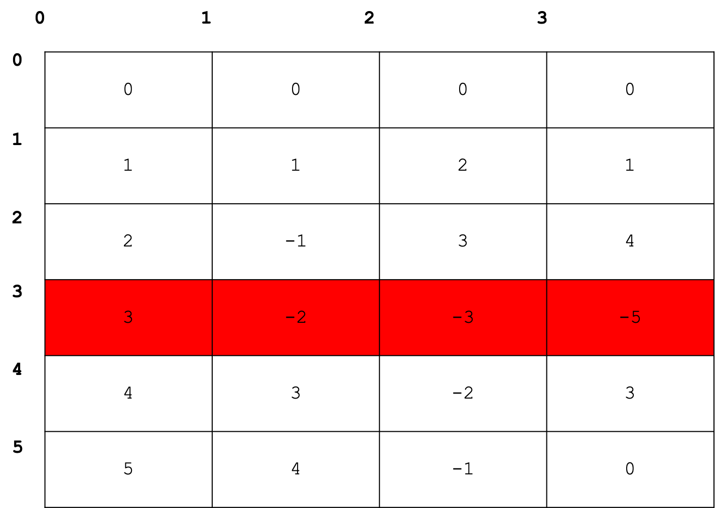
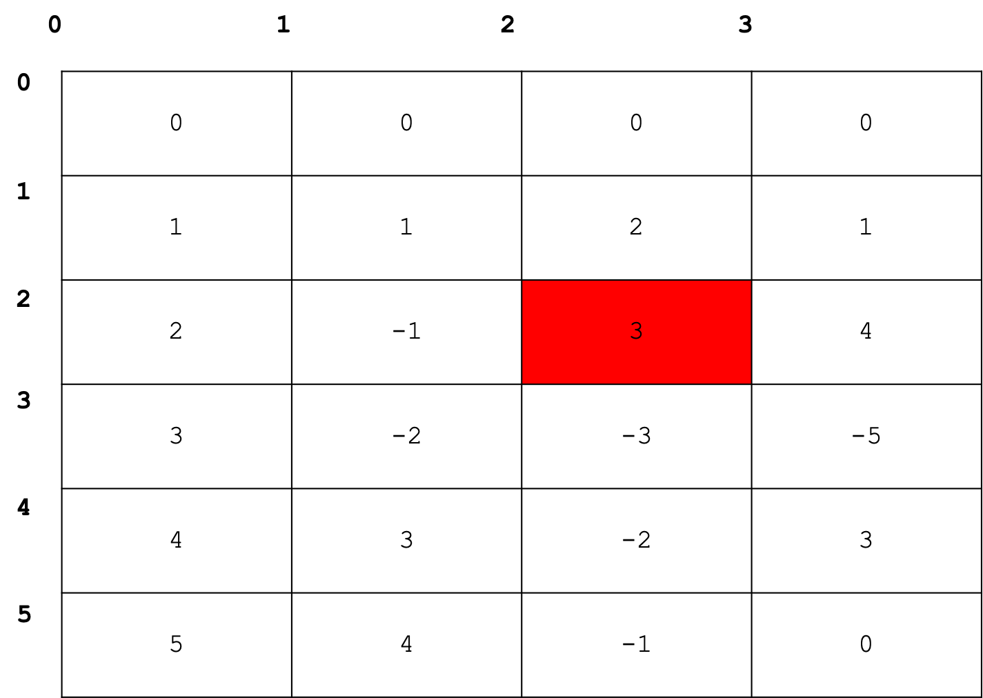
which indicates the particle was at [-2,-3,-5] after three seconds. If one wished to know the y coordinate after two seconds, one could use
trajectory[2][2]
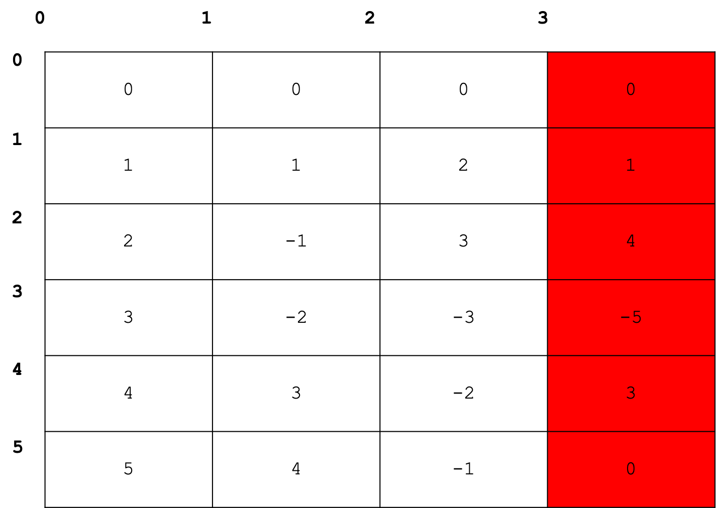
If, for some reason, we wished to study the trajectory along the z coordinate only then NumPy allows us to access this information easily using
trajectory[:,3]
Exercise: Using the boiling point data for ethanol, displayed below, use a one-dimensional array to determine the mean and median of the experimental data collected.
| Experiment | Boiling Point ($^{\circ}$C) |
|---|---|
| 1 | 78.1 $\pm$ 0.1 |
| 2 | 78.8 $\pm$ 0.1 |
| 3 | 78.4 $\pm$ 0.1 |
| 4 | 78.6 $\pm$ 0.1 |
| 5 | 78.4 $\pm$ 0.1 |
| 6 | 77.9 $\pm$ 0.1 |
| 7 | 79.4 $\pm$ 0.1 |
| 8 | 78.0 $\pm$ 0.1 |
| 9 | 78.7 $\pm$ 0.1 |
| 10 | 78.4 $\pm$ 0.1 |
Following this, create a 3 x 3 array for the coordinates of the atoms in a molecule of carbon dioxide displayed below
| Atom | x / Angstroms | y / Angstroms | z / Angstroms |
|---|---|---|---|
| C | 0 | 0 | 0 |
| 01 | -1.16 | 0 | 0 |
| 02 | 0 | 0 | +1.16 |
# Write your code here
For functions that are not built into an imported module you will be required to write your own. In the following tutorial you will learn how to do just this so that you can computationally solve any problem that may come your way.
A note on NumPy
This has been a very brief introduction to NumPy. The NumPy module has a lot more to offer than is described here. In future tutorials more of the NumPy module's functionality will be introduced.