
Prerequisites:
- containers
- numpy
- matplotlib
matplotlib is a powerful tool that allows multidimensional data to be visualised. We will start with a simple scatter plot and build up to two dimensional surface plots.
import numpy as np
import matplotlib.pyplot as plt
x = np.linspace(-4, 4, 20)
y = np.linspace(-4, 4, 20)

plt.scatter(x, y)
plt.show()
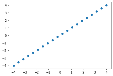
In the above cell we generated two one dimensional numpy arrays, consisting of 20, evenly spaced numbers between -4 and 4. We then plotted these two arrays as a scatter plot.
Plotting two dimensional data
There are many examples where multidimensional plots become useful, the most common is an energy landscape. An energy landscape is a mapping of possible states of a system. This concept is frequently used in physics, chemistry, biology e.g. to describe the possible conformations of atoms in a system as a function of conformational energy.
In this example, we are going to plot a simple function.
$z = x^2 + y^2$
def xs_plus_ys(x, y):
    """
    Calculates
    """
    z = x ** 2 - y ** 2
    return z

x_grid, y_grid = np.meshgrid(x, y) # Generate two grids of x and y values
z = xs_plus_ys(x_grid, y_grid) # Calculate the x**2 + y**2

plt.scatter(x_grid, y_grid, c=z) # Plot the x and y grids and color the points based upon x**2 + y**2
plt.xlabel("x axis") # Label the x axis
plt.ylabel("y axis") # Label the y axis
plt.show() # Display the plot
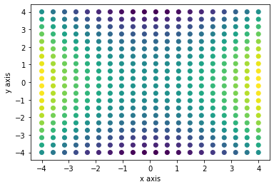
np.meshgrid is a numpy library that generates a nxn grid out of two one dimensional arrays. We have generated two multidimensional arrays that corespond to all x and y positions within a two dimensional grid. We then use the function xs_plus_ys to generate the $x^2 + y^2$ values.
This data can be plotted as a scatter plot, with each plot being colored based upon its z value, using the optional arguement c. However this can be difficult to visualise and matplotlib has many built in funcitons to help visualise this data. Below is an example of the contour method in matplotlib.
contours = plt.contour(x_grid, y_grid, z) # Plot x**2 + y**2
plt.clabel(contours) # Add labels to each contour
plt.xlabel("x axis") # Label the x axis
plt.ylabel("y axis") # Label the y axis
plt.show() # Display the plot

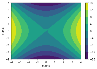
matplotlib's contourf functions is similiar to the contour function except it fills the space between contour lines. Thus instead of lines which seperate individual regions, there are shaded areas.
plt.contourf(x_grid, y_grid, z) # Plot x**2 + y**2
plt.xlabel("x axis") # Label the x axis
plt.ylabel("y axis") # Label the y axis
plt.show() # Display the plot

These colors represent a third dimension and it is useful to have a scale that shows the numerical that each color represents. This is achieved with a colorbar. Colorbars are added to the plot with the plt.colorbar() method.
plt.contourf(x_grid, y_grid, z) # Plot x**2 + y**2
plt.colorbar()
plt.xlabel("x axis") # Label the x axis
plt.ylabel("y axis") # Label the y axis
plt.show() # Display the plot
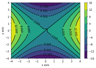
It is possible to combine these plots and have contour lines as well as the shaded regions.
contours = plt.contour(x_grid, y_grid, z, colors="black")
plt.clabel(contours)
plt.contourf(x_grid, y_grid, z)
plt.colorbar()
plt.xlabel("x axis")
plt.ylabel("y axis")
plt.show()
Customising plots
As you will learn, there are many ways to customise plots in matplotlib. There are a few useful ways customise contour plots.
- Both contour and contourf functions have an optional variable called levels which controls the the gap between contour levels.
- Many colormaps exist and can be altered with the optional variable cmap. *
color_levels = np.array([-20, -10, 0, 10, 20])

contours = plt.contour(x_grid, y_grid, z, colors="black", levels=color_levels, )
plt.clabel(contours)
plt.contourf(x_grid, y_grid, z, levels=color_levels, cmap="Blues")
plt.colorbar()

plt.xlabel("x axis")
plt.ylabel("y axis")
plt.show()
