
Numerical Integration Methods#
In molecular dynamics, we apply this general procedure to model the trajectories of atoms and molecules. Starting with the positions and velocities of all atoms at time \(t\), we calculate the forces acting on each atom (and thus their accelerations), then use approximate versions of the equations of motion to predict the atomic positions and velocities a short time later. By iteratively repeating this process we generate a sequence of positions and velocities that describes the dynamics of the atoms as a function of time. This process of stepping forward in time using approximate solutions to differential equations is called numerical integration.
While the same general process applies to all molecular dynamics, the quality of our simulation, and the degree to which we need to balance computational cost with accuracy, depends critically on our choice of approximation for the equations of motion. The simplest approach, known as Euler’s method, helps us understand both the basics of numerical integration and its potential pitfalls.
Euler’s Method#
The simplest approach to solving the equations of motion is Euler’s method.
For a given timestep \(\Delta t\), we can approximate the new positions and velocities as:
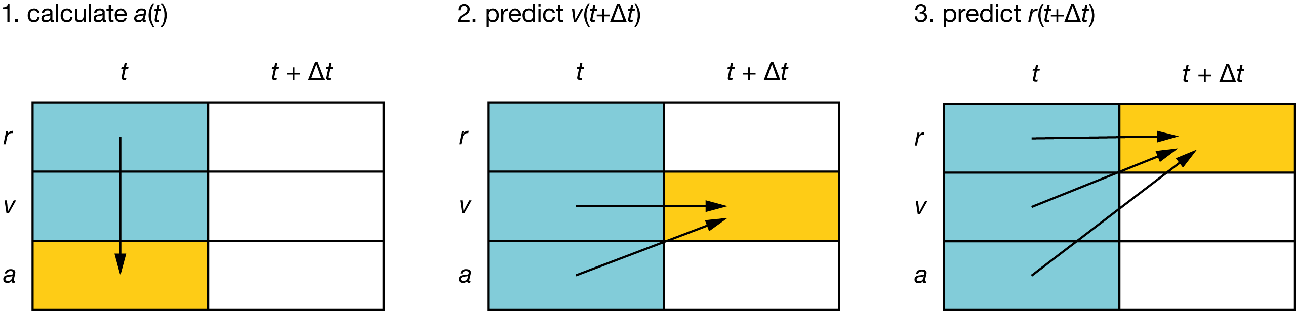
Fig. 7 Schematic showing the sequence of calculations performed each step of a molecular dynamics simulation, using Euler’s method:
#
\(a(t)\) is calculated from \(r(t)\) (via \(F(r)\));
\(v(t+\Delta t)\) is calculated using \(v(t)\) and \(a(t)\);
\(r(t+\Delta t)\) is calculated using \(r(t)\), \(v(t)\), and \(a(t)\).
While Euler’s method is straightforward to understand and implement, it has significant drawbacks. The method effectively assumes that forces and velocities remain constant over each timestep: we predict \(r(t+\Delta t)\) and \(v(t+\Delta t)\) using only \(a(t)\) and \(v(t)\). In reality, both acceleration and velocity change continuously as our system moves across the potential energy surface.
This approximation leads to two key problems. First, the method introduces small systematic errors at each step between the predicted changes in \(v\) and \(r\) and the changes that would occur if we could integrate the equations of motion exactly. These errors accumulate over time, causing the total energy (kinetic plus potential) to drift rather than remain constant as it should.
Second, the equations are not time reversible. In principle, molecular motion should be reversible — if we could exactly reverse all velocities at any point, our system should retrace its path. Euler’s method breaks this physical principle. If we take a step forward in time and then reverse all velocities, the Euler equations will not return our system to its starting point. This is because the forward step uses information only from the beginning of the timestep, while a backward step would use information from the end of the timestep. This asymmetry means that forward and backward steps follow different trajectories, violating the fundamental time-symmetry of molecular motion.
The Velocity Verlet Method#
A much better approach, commonly used in practical Molecular Dynamics codes, is the velocity Verlet algorithm. This method proceeds in several steps:
First, update positions:
Then calculate velocities at the half-step:
Update accelerations using the new positions:
Finally, complete the velocity update:
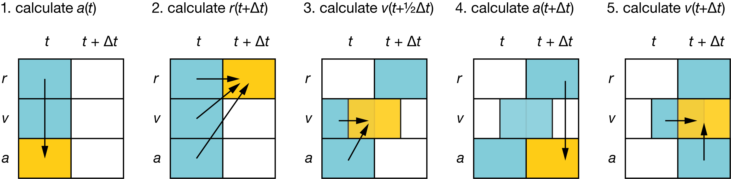
Fig. 8 Schematic showing the sequence of calculations performed each step of a molecular dynamics simulation, using the Velocity Verlet method:
#
\(a(t)\) is calculated from \(r(t)\) (via \(F(r)\));
\(r(t+\Delta t)\) is calculated using \(r(t)\), \(v(t)\), and \(a(t)\);
\(v(t+\frac{1}{2}\Delta t)\) is calculated using \(v(t)\) and \(a(t)\);
\(a(t+\Delta t)\) is calculated using \(r(t+\Delta t)\);
\(v(t+\Delta t)\) is calculated using \(v(t+\frac{1}{2}\Delta t)\) and \(a(t+\Delta t)\).
In practice, we can simplify this implementation by avoiding explicit calculation of the half-step velocities, leading to three essential equations:
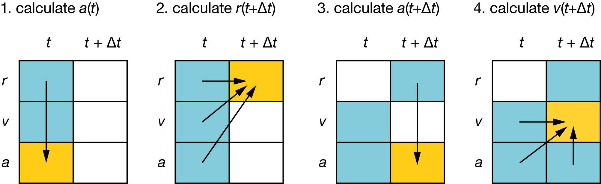
Fig. 9 Schematic showing the sequence of calculations performed each step of a molecular dynamics simulation, using the simplified Velocity Verlet method:
#
\(a(t)\) is calculated from \(r(t)\) (via \(F(r)\));
\(r(t+\Delta t)\) is calculated using \(r(t)\), \(v(t)\), and \(a(t)\);
\(a(t+\Delta t)\) is calculated using \(r(t+\Delta t)\);
\(v(t+\Delta t)\) is calculated using \(v(t)\), \(a(t)\), and \(a(t+\Delta t)\).
This algorithm provides much better numerical accuracy and properly conserves energy, making it far more suitable for molecular dynamics simulations.