Monte Carlo Simulation of the 1D Ising Model

In this exercise, you’ll implement a Monte Carlo simulation of a 1D Ising model with 4 spins and periodic boundary conditions. We’ll build this up in steps, eventually calculating the mean magnetisation as a function of temperature.

The one-dimensional Ising model consists of a line of spins that can each take values \(\sigma_i = \pm1\) (up or down). The total energy of the system depends on the relative orientations of neighbouring spins, according to:

\[H(\sigma) = -\sum_{<ij>} J_{ij}\sigma_i\sigma_j\]

where the sum runs over adjacent pairs \(i\) and \(j\) and \(J_{ij}\) is the coupling constant between spins \(i\) and \(j\).

Consider a simple model system with only four spins. We make our system periodic so that spins 1 and 4 are neighbours (every spin neighbours two other spins).

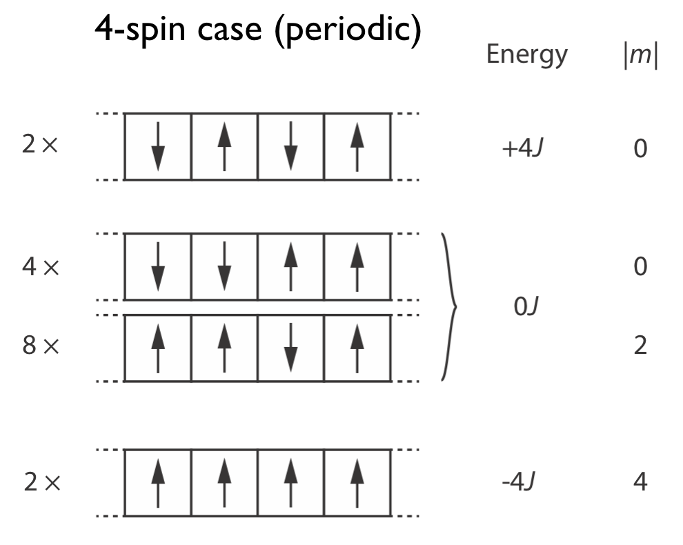
This system has a total of \(2^4=16\) spin states. There are two degenerate states with all spins parallel, with enegy \(-4J\), two degenerate states with alternating up and down spins, with energy \(+4J\), and 12 degenerate states with both parallel and anti-parallel adjacent spins: these all have energy \(0J\). For each of these spin states we can also calculate the total magnetisation, \(|m|\), as the difference between the numbers of up and down spins.

Fig. 12 The four inequivalent states of a 4-spin Ising model, showing their spin configurations, energies, and magnetisation.

Consider the problem of calculating the average absolute magnetisation \(\left<M\right>\) as a function of temperature? Four our 4-spin system we can compute this directly using statistical mechanics:

\[\left<M\right> = \sum_i \frac{\left|m_i\right|g_i\exp\left(-E_i/kT\right)}{Z}\]

where \(Z\) is the usual partition function \(Z = \sum_i \exp\left(-E_i/kT\right)\), and \(g_i\) is the degeneracy of the \(i\)^th state.

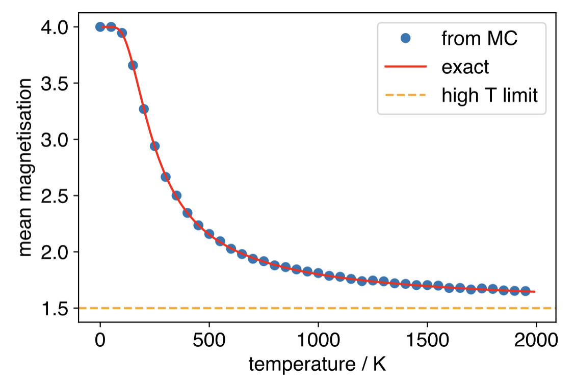
For example, evaluating this gives \(\left<M\right> = 1.5\) in the high-T limit (\(T\to\infty\)).

You can also numerically simulate this system using Metropolois Monte Carlo.

Part 1. Energy Calculation

Write a function that calculates the energy of a periodic 1D Ising model. You should represent the spin-state of your system using a numpy array where every element is either \(+1\) (spin-up) or \(-1\) (spin-down). Your function will take as input a single spin state and \(J\). Test your function by passing the following numpy arrays, which correspond to the four inequivalent spin configurations of a 4-spin system (Use \(J = 0.012\) eV).:

np.array([-1,1,-1,1]) # E = +4J
np.array([-1,-1,1,1]) # E = 0J
np.array([1,1,-1,1])  # E = 0J
np.array([1,1,1,1])   # E = -4J

Part 2: Single Monte Carlo Step

Implement a single MC step that:

1. Picks a random spin.

2. Calculates \(\Delta E\) for flipping this spin.

3. Accepts/rejects the flip using the Metropolis criterion.

Python Hints

1. One way that you can select a random element from a numpy array is using np.random.randint(), which generates random integers from a specified range. By setting that range to the length of an array, you can use the result to pick a random array element.

my_array = np.array(['a', 'b', 'c', 'd']) # create an length-4 array
random_index = np.random.randint(len(my_array)) # generate a random integer between 0 and 3
print(my_array[random_index]) # print the corresponding array element

2. Remember that a spin flip corresponds to changing a spin from \(+1\) to \(-1\), or from \(-1\) to \(+1\). In both cases, this corresponds to multiplying that element of your spin-state array by \(-1\).

3. Creating copies of numpy arrays requires care:

import numpy as np

original_array = np.array(['a', 'b', 'c'])
copied_array = original_array
copied_array[0] = 'z'

print(f'original array: {original_array}')
print(f'copied array: {copied_array}')

original array: ['z' 'b' 'c']
copied array: ['z' 'b' 'c']

Changing the first element in copied_array changed original_array too. Why does this happen?

The assignment copied_array = original_array does not create a new array. Instead, both it creates a new variable name that points at the same data in memory. Because original_array and copied_array both point to the same data, any changes to one array appear to be mirrored by the other array.

For a true copy, use the copy() method:

original_array = np.array(['a', 'b', 'c'])
copied_array = original_array.copy()  # Create a true copy
copied_array[0] = 'z'

print(f'original array: {original_array}')
print(f'copied array: {copied_array}')

original array: ['a' 'b' 'c']
copied array: ['z' 'b' 'c']

For the Ising model, you’ll need to:

1. Try flipping a spin

2. Calculate the energy change

3. Accept the flip or keep the previous state

Without copy(), you can run into trouble:

# Problem: both variables point to same data
spins = np.ones(4)
new_spins = spins   # Seems like we are copying the spin state, but we are not
new_spins[0] *= -1     # Flip a spin
print(f'proposed move: {new_spins}')
print(f'old spins: {spins}')  # Changed too!

# Solution: make a true copy
spins = np.ones(4)
new_spins = spins.copy()
new_spins[0] *= -1
print(f'proposed move: {new_spins}')
print(f'old spins: {spins}')  # Stays unchanged

proposed move: [-1.  1.  1.  1.]
old spins: [-1.  1.  1.  1.]
proposed move: [-1.  1.  1.  1.]
old spins: [1. 1. 1. 1.]

Part 3: Magnetisation

The magnetisation is simply the sum of the spins. Implement a function to calculate the absolute magnetisation per spin. Your function should take a single numpy array describing the spin-state as the argument.

Part 4: Full Simulation

Now combine these pieces to simulate the system at 1000 K.

1. Perform \(N\) MC steps, where each step you propose a random spin flip and accept or reject using the Metropolis criterion

2. For each step, whether you accept or reject the move, calculate the magnetisation.

3. Your mean magnetisation is then the mean value over all MC steps. As for the previous exercise, your calculation will progressively converge its estimate of \(\left<M\right>\) as you increase the number of MC steps. Evaluate what a reasonable value of \(N\) is to converge your estimate of the mean magnetisation to 2 decimal places.

Note: You can start your simulation from a specified spin-state (e.g., [1, 1, 1, 1]) or from a random spin-state, using np.random.choice([1,-1], size=N where N is the size of the array you want to generate.

Part 5: Temperature Dependence

Wrap your entire simulation in a function that takes as arguments the temperature \(T\) and \(J\). By calling this function from a loop, run simulations at a range of temperatures from 0 K to 2000 K. Plot the mean magnetisation versus temperature, and compare to the high-temperature limit value.

(Bonus: write a function to calculate the exact magnetisation using the statistical mechanical expression given above. Plot this exact result on the same plot as your simulation data to compare the two.)

Fig. 13 Plot of mean magnetisation for a 4-spin Ising model (\(J\) = 0.012 eV) as a function of temperature, calculated using Metropolis Monte Carlo and compared to the exact result.