Estimating \(\pi\)#
To understand the principles of Monte Carlo methods, let us consider a simple problem: calculating the area of a circle and thus the value of \(\pi\). Analytically, we can find the area of a circle by imagining it divided into thin concentric rings. The area of each ring is its circumference (\(2\pi r\)) multiplied by its thickness (\(\Delta r\)).
Adding up all of these areas gives
In the limit that each ring becomes infinitesimally thin, \(\Delta r \to \mathrm{d}r\), this approximate sum becomes an exact integral
What if we could not perform this integration analytically? An alternative approach is to estimate the area of the circle using random sampling.
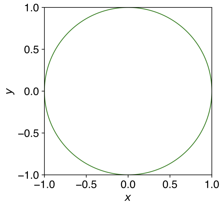
Consider a unit circle (\(R=1\)) inscribed in a \(2\times2\) square. The ratio of their areas is:

Fig. 11 A circle of radius \(R=1\) inside a \(2\times2\) square. The area of the circle is \(\pi R^2\), and the area of the square is \(2\times2 = 4\). Hence we can define \(\pi\) as \(\frac{4A_\mathrm{circle}}{A_\mathrm{square}}\).#
We can estimate this ratio — and thus \(\pi\) — using random sampling. This demonstrates a key principle of Monte Carlo integration: we can approximate integrals by randomly sampling the integration space and counting the fraction of samples that meet certain criteria.
Exercise 1#
Your task is to implement a Monte Carlo estimation of \(\pi\) using random sampling. The general approach is this:
We generate a series of points with random \((x,y)\) values that are uniformly distributed over our \(2\times2\) square.
The ratio of points that lie inside the unit circle to the total number of points gives us an estimate for \(A_\mathrm{circle}/A_\mathrm{square}\).
This can then be used to estimate \(\pi\), via \(A_\mathrm{circle}/A_\mathrm{square} = \pi/4\).
You can generate random pairs of numbers between \(-1\) and \(+1\) with the following numpy code:
import numpy as np

N = 50 # Generate 50 pairs of random numbers
points = np.random.uniform(low=-1, high=1, size=(N,2))
Write a function that takes an integer argument \(N\) and returns \(N\) pairs of random points with \(-1.0\leq x \leq1.0\) and \(-1.0 \leq y \leq 1.0\)
Use the code below to plot your random points.
import matplotlib.pyplot as plt
%config InlineBackend.figure_format='retina'

def plot_random_points(points):
    # Set up the plot with circle
    plt.axes()
    circle = plt.Circle((0,0), radius=1.0, fc='white', ec="green")
    plt.gca().add_patch(circle)
    plt.axis('scaled')
    plt.xlim(-1.0, 1.0)
    plt.ylim(-1.0, 1.0)
    plt.xlabel(r"$x$")
    plt.ylabel(r"$y$")

    # plot the points, using different colours depending on whether they
    # are inside or outside the circle
    for x, y in points:
        if x**2 + y**2 < 1.0:
            plt.plot(x, y, 'o', color='red', alpha=0.5, markersize=5)
        else:
            plt.plot(x, y, 'o', color='blue', alpha=0.5, markersize=5)

    plt.show()
Write a function that takes as input your randomly generated points and calculates the proportion that are inside the unit circle, i.e. \(x^2 + y^2 \leq 1\).
Write a function that takes as input the number of points to sample, that calls your two functions above to (a) generate \(N\) points, and (b) calculates the proportion inside the circle. Your function should then estimate \(\pi\) and return this estimate.
How does the accuracy of your estimate change for \(N\) = 50, 500, 5000, 50000 points?
What happens if you rerun the code with the same value of \(N\)?
Write another wrapper function that performs \(M\) Monte Carlo calculations (each with \(N\) points). This function should take two arguments, \(N\) and \(M\). Use this function to estimate the mean and standard deviation of your estimate of \(\pi\) for \(N\) = 50, 500, 5000, 50000 samples.
