Function minimisation

The potential energy surface describes the energy as a function of the atomic configuration in space. In computational chemistry, frequently the aim is to study the minimum energy atomic configuration. Therefore, we must be able to find the minimum of a given potential energy surface.

In this section, we will consider the simple case of a potential energy surface of two atoms interacting in space, in particular argon atoms. This is typically modelled with a Lennard-Jones potential, which aims to describe the long-range attractive London dispersion forces between the two atoms and the short-range repulsive Pauli exclusion principle (that two atoms cannot occupy the same space). The functional form of the Lennard-Jones potential is as follows,

\[ E(r_{ij}) = \frac{A}{r_{ij}^{12}} - \frac{B}{r_{ij}^6}, \]

where \(E(r_{ij})\) is the potential energy, \(r_{ij}\) is the distance between atoms \(i\) and \(j\), and \(A\) and \(B\) are interaction specific constants. The first part of the above equation describes the repulsive interaction, while the second describes the attractive (remember that a negative energy contribution describes an attraction). We can plot a typical Lennard-Jones potential as shown below.

import numpy as np
import matplotlib.pyplot as plt

A = 1e5
B = 40

r = np.linspace(3.5, 10, 100)
plt.plot(r, A / (r ** 12) - B / (r ** 6))
plt.xlabel('$r_{ij}$/Å')
plt.ylabel('$E$/eV')
plt.show()

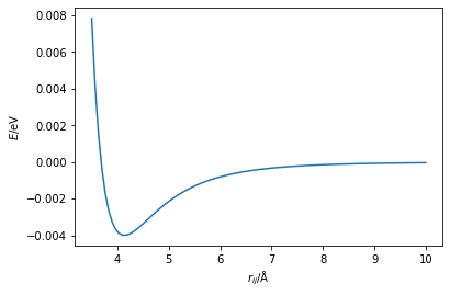
In the above plot, we can see where the energy is minimised, at around 4.1 Å. Function minimisation aims to enable a computational algorithm to find this also. For this, we use minimisation algorithms, which typically use the local gradient and curvature to determine the shape of the function, such that any moves are downhill. Collectively, these algorithms are known as gradient-descent methods.