Exercises

The first exercise is to write a function to calculate the distance between two atoms and use it in the nested loop featured previously.

import numpy as np

def distance(atom1, atom2):
    """
    Find the distance between two atoms. 
    
    Args:
        atom1 (array_like): x, y, z coordinates of atom 1.
        atom2 (array_like): x, y, z coordinates of atom 2.
    
    Returns:
        (float): distance between atoms 1 and 2.
    """
    return np.sqrt(np.sum((atom1 - atom2) ** 2))

atom_1 = [0.1, 0.5, 3.2]
atom_2 = [0.4, 0.5, 2.3]
atom_3 = [-0.3, 0.3, 1.7]

distances = []

atoms = np.array([atom_1, atom_2, atom_3])
for i, a_i in enumerate(atoms):
    for j, a_j in enumerate(atoms[i+1:]):
        distances.append(distance(a_i, a_j))
        
print(distances)

[0.9486832980505141, 1.5652475842498532, 0.9433981132056602]

The second exercise is to write a function that implements the second-order rate equation.

def second_order(t, A0, k):
    """
    The second order rate law. 
    
    Args: 
        t (float): Time (s).
        A0 (float): Initial concentration (M).
        k (float): Rate constant (M-1s-1).
    
    Returns:
        (float): Concentration at time t (M).
    """
    return A0 / (A0 * k * t + 1)

We are to then plot the data given in the table as a scatter plot and overlay the model second order rate equation over this using the different parameter sets.

import matplotlib.pyplot as plt

t = np.array([0, 600, 1200, 1800, 2400])
At = np.array([0.400, 0.350, 0.311, 0.279, 0.254])

x = np.linspace(0, 2400, 1000)

plt.plot(t, At, 'o')
plt.plot(x, second_order(x, 0.6, 0.006), label='1')
plt.plot(x, second_order(x, 0.4, 0.0006), label='2')
plt.plot(x, second_order(x, 0.2, 0.6), label='3')
plt.xlabel('Time/s')
plt.ylabel('$[$A$]_t$')
plt.legend()
plt.show()

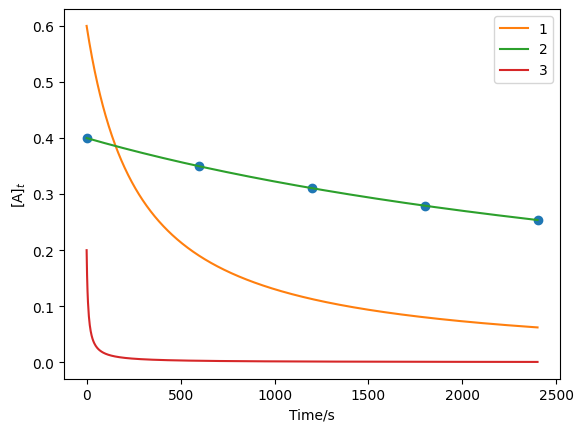
We can see that the model labeled as 2 offers the best agreement to the data.