LaTeX Formatting

In scientific writing, you need to format mathematical expressions, chemical formulae, and units correctly. Jupyter notebooks and matplotlib both use LaTeX notation for mathematical typesetting.

Mathematical Expressions in Markdown

To write mathematical expressions in markdown cells, wrap them in dollar signs $...$ for inline mathematics or $$...$$ for displayed equations.

Basic syntax:

You type	You get
$x_i$	\(x_i\)
$x^2$	\(x^2\)
$\alpha$, $\beta$, $\Delta$	\(\alpha\), \(\beta\), \(\Delta\)
$\frac{a}{b}$	\(\frac{a}{b}\)
$E = mc^2$	\(E = mc^2\)

If you need help with LaTeX syntax, AI assistants like ChatGPT or Claude are very good at generating the correct LaTeX markup for mathematical expressions.

Example:

The Arrhenius equation is $k = A e^{-E_a/RT}$.

Renders as:

The Arrhenius equation is \(k = A e^{-E_a/RT}\).

Chemical Formulae and Equations

Chemical formulae should be typeset in upright (non-italic) text, not as mathematical variables: e.g., H₂O, rather than \(H_2O\).

There are two approaches:

Using LaTeX \mathrm{}

The \mathrm{} command produces upright (non-italic) text in math mode:

You type	You get
$\mathrm{H_2O}$	\(\mathrm{H_2O}\)
$\mathrm{CO_2}$	\(\mathrm{CO_2}\)
$\mathrm{NaCl}$	\(\mathrm{NaCl}\)
$\mathrm{H_2SO_4}$	\(\mathrm{H_2SO_4}\)

Using HTML

Alternatively, you can use HTML tags for subscripts and superscripts:

Note that HTML uses a hyphen (-) rather than a proper minus sign (−). You can use − for a proper minus sign in HTML, but LaTeX handles this correctly by default, making it often the simpler choice.

You type	You get
H<sub>2</sub>O	H2O
CO<sub>2</sub>	CO2
10<sup>-3</sup> mol dm<sup>-3</sup>	10-3 mol dm-3

HTML tags work in markdown cells but not in matplotlib labels.

LaTeX in Matplotlib Labels

The same LaTeX syntax used in markdown cells works in matplotlib labels. Wrap mathematical expressions in dollar signs $...$.

import numpy as np
import matplotlib.pyplot as plt
%config InlineBackend.figure_format='retina'

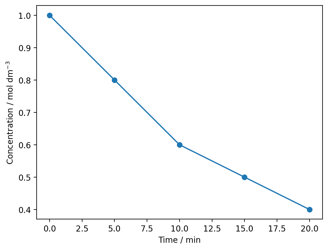
time = np.array([0, 5, 10, 15, 20])
concentration = np.array([1.0, 0.8, 0.6, 0.5, 0.4])

plt.plot(time, concentration, 'o-')
plt.xlabel('Time / min')
plt.ylabel('Concentration / mol dm$^{-3}$')
plt.show()

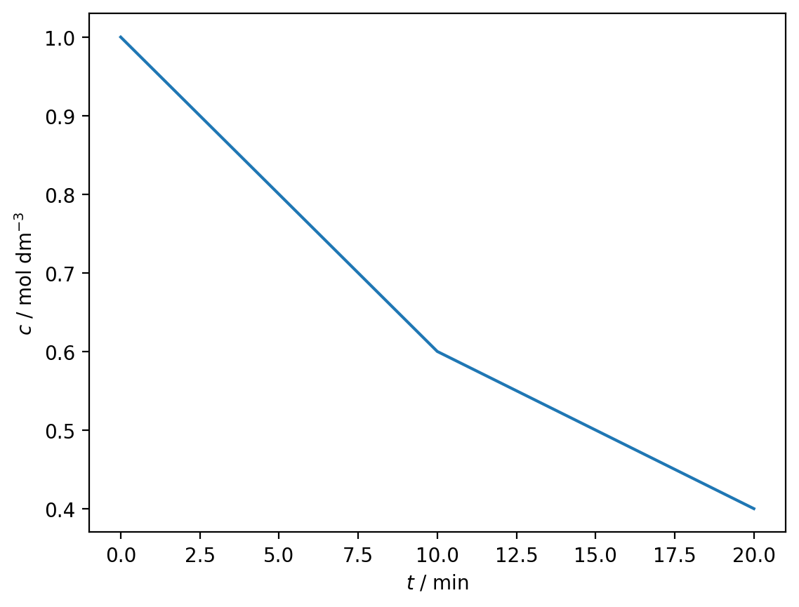
Variables in labels should be italicised by wrapping them in $...$:

plt.plot(time, concentration)
plt.xlabel('$t$ / min')
plt.ylabel('$c$ / mol dm$^{-3}$')
plt.show()

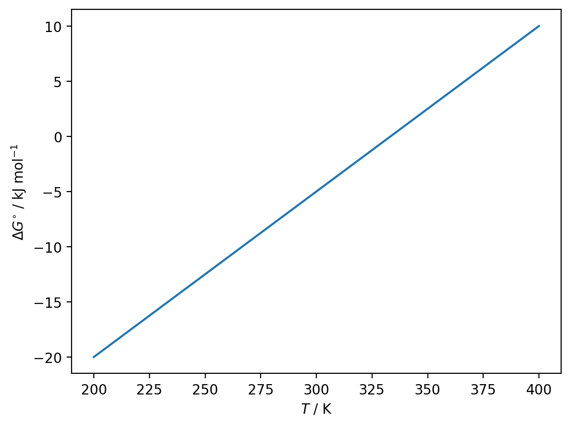
For expressions containing backslashes (like Greek letters or special commands), use the r prefix to create a “raw” string. This prevents Python from interpreting the backslashes:

temperature = np.linspace(200, 400, 50)
delta_G = -50 + 0.15 * temperature

plt.plot(temperature, delta_G)
plt.xlabel(r'$T$ / K')
plt.ylabel(r'$\Delta G^{\circ}$ / kJ mol$^{-1}$')
plt.show()

Exercise

Create a plot showing the relationship between inverse temperature and the natural logarithm of the rate constant (an Arrhenius plot).

Use this data:

inverse_temp = np.array([0.0025, 0.0027, 0.0029, 0.0031, 0.0033])  # K^-1
ln_k = np.array([-8.5, -7.8, -7.2, -6.7, -6.2])

Your plot should have:

1. x-axis label: \(T^{-1}\) / K\(^{-1}\) (with proper formatting)

2. y-axis label: ln \(k\) (with \(k\) italicised)

3. A title: “Arrhenius Plot”

Show solution

inverse_temp = np.array([0.0025, 0.0027, 0.0029, 0.0031, 0.0033])
ln_k = np.array([-8.5, -7.8, -7.2, -6.7, -6.2])

plt.plot(inverse_temp, ln_k, 'o-')
plt.xlabel(r'$T^{-1}$ / K$^{-1}$')
plt.ylabel(r'ln $k$')
plt.title('Arrhenius Plot')
plt.show()

Summary

You have learned how to:

• Write mathematical expressions in markdown using $...$

• Format subscripts with _ and superscripts with ^

• Use Greek letters and fractions in LaTeX notation

• Format chemical formulae correctly using \mathrm{}

• Apply the same LaTeX syntax to matplotlib labels

• Use raw strings (r'...') for expressions containing backslashes