
Worked Examples: Gradient Descent Method#
These worked solutions correspond to the exercises on the Gradient Descent Method page.
How to use this notebook:
Try each exercise yourself first before looking at the solution
The code cells show both the code and its output
Download this notebook if you want to run and experiment with the code yourself
Your solution might look different - that’s fine as long as it gives the correct answer!
Exercise: Fixed Step Size Gradient Descent#
Problem: Implement gradient descent with a fixed step size to find the minimum of the harmonic potential energy surface. We need to first write a function to calculate the first derivative of the harmonic potential:
Then implement the gradient descent algorithm using:
We’ll start from \(r = 1.0\) Å and explore how different step sizes affect convergence.
Setup: Define functions#
First, we’ll define our harmonic potential and its derivative:
import numpy as np
import matplotlib.pyplot as plt

%config InlineBackend.figure_format='retina'
def harmonic_potential(r, k, r_0):
    """Calculate the harmonic potential energy.

    Args:
        r (float): Bond length (Å). Can be a float or np.ndarray.
        k (float): Force constant (eV Å^-2).
        r_0 (float): Equilibrium bond length (Å).

    Returns:
        Potential energy (eV). Type matches input r.
    """
    return 0.5 * k * (r - r_0) ** 2

def harmonic_gradient(r, k, r_0):
    """Calculate the first derivative of the harmonic potential.

    Args:
        rr (float): Bond length (Å). Can be a float or np.ndarray.
        k (float): Force constant (eV Å^-2).
        r_0 (float): Equilibrium bond length (Å).

    Returns:
        First derivative dU/dr (eV Å^-1). Type matches input r.
    """
    return k * (r - r_0)
# Parameters for H₂
k = 36.0  # eV Å^-2
r_0 = 0.74  # Å

# Test the gradient function
r_test = 1.0  # Å
gradient = harmonic_gradient(r_test, k, r_0)
print(f"Gradient at r = {r_test} Å: U'(r) = {gradient:.3f} eV Å^-1")
Gradient at r = 1.0 Å: U'(r) = 9.360 eV Å^-1
Part 1: Fixed step size Δr = 0.01 Å#
Let’s implement the gradient descent algorithm with a small step size and see how it performs:
# Gradient descent parameters
r_start = 1.0  # Å
delta_r = 0.01  # Å (step size)
max_iterations = 50
convergence_threshold = 0.001  # eV Å⁻¹

# Initialize
r_current = r_start
r_history = [r_current]
gradient_history = []

print(f"Starting gradient descent with Δr = {delta_r} Å\n")
print("Iteration | Position (Å) | Gradient (eV Å⁻¹)")
print("-" * 50)

converged = False
for iteration in range(max_iterations):
    # Calculate gradient at current position
    gradient = harmonic_gradient(r_current, k, r_0)
    gradient_history.append(gradient)

    print(f"{iteration:9d} | {r_current:12.6f} | {gradient:18.6f}")

    # Check for convergence
    if abs(gradient) < convergence_threshold:
        print(f"\nConverged after {iteration} iterations!")
        print(f"Final position: r = {r_current:.6f} Å")
        print(f"Analytical solution: r₀ = {r_0} Å")
        print(f"Error: {abs(r_current - r_0):.6f} Å")
        converged = True
        break

    # Update position (gradient descent step)
    r_current = r_current - delta_r * np.sign(gradient)
    r_history.append(r_current)

if not converged:
    print(f"\nDid not converge within {max_iterations} iterations.")
    print(f"Final position: r = {r_current:.6f} Å")
    print(f"Final gradient: {gradient:.6f} eV Å⁻¹")
Starting gradient descent with Δr = 0.01 Å

Iteration | Position (Å) | Gradient (eV Å⁻¹)
--------------------------------------------------
        0 |     1.000000 |           9.360000
        1 |     0.990000 |           9.000000
        2 |     0.980000 |           8.640000
        3 |     0.970000 |           8.280000
        4 |     0.960000 |           7.920000
        5 |     0.950000 |           7.560000
        6 |     0.940000 |           7.200000
        7 |     0.930000 |           6.840000
        8 |     0.920000 |           6.480000
        9 |     0.910000 |           6.120000
       10 |     0.900000 |           5.760000
       11 |     0.890000 |           5.400000
       12 |     0.880000 |           5.040000
       13 |     0.870000 |           4.680000
       14 |     0.860000 |           4.320000
       15 |     0.850000 |           3.960000
       16 |     0.840000 |           3.600000
       17 |     0.830000 |           3.240000
       18 |     0.820000 |           2.880000
       19 |     0.810000 |           2.520000
       20 |     0.800000 |           2.160000
       21 |     0.790000 |           1.800000
       22 |     0.780000 |           1.440000
       23 |     0.770000 |           1.080000
       24 |     0.760000 |           0.720000
       25 |     0.750000 |           0.360000
       26 |     0.740000 |          -0.000000

Converged after 26 iterations!
Final position: r = 0.740000 Å
Analytical solution: r₀ = 0.74 Å
Error: 0.000000 Å
Explanation:
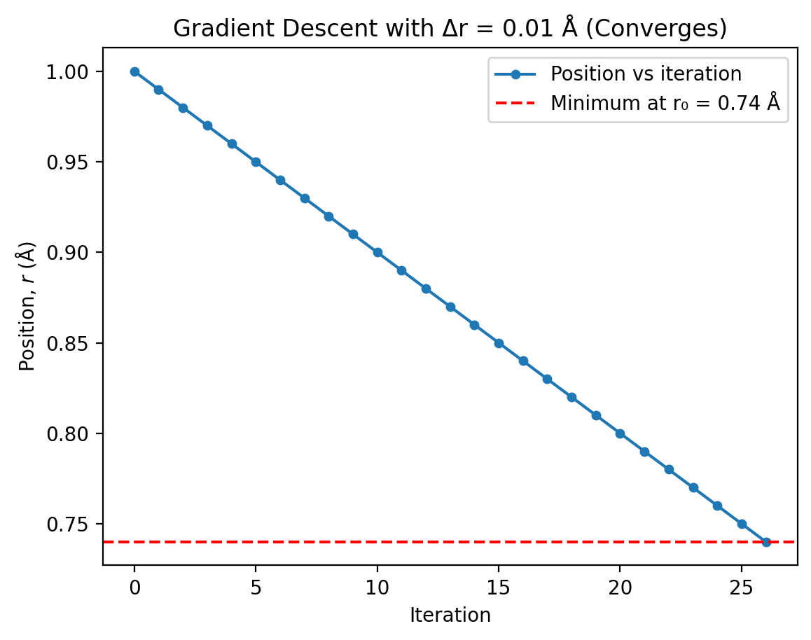
With \(\Delta r = 0.01\) Å, the algorithm converges successfully in 26 iterations. Key observations:
Steady convergence: The position moves consistently towards the minimum at \(r_0 = 0.74\) Å.
Fixed step size: Each iteration moves exactly 0.01 Å in the direction indicated by the gradient sign:
When \(r > r_0\): gradient is positive, so we step left (decrease \(r\))
When \(r < r_0\): gradient is negative, so we step right (increase \(r\))
Final accuracy: The algorithm stops when \(|U'(r)| < 0.001\) eV Å⁻¹, which occurs at approximately \(r = 0.74\) Å—exactly the analytical minimum!
Why 26 iterations?: Starting at \(r = 1.0\) Å, we need to travel \(0.26\) Å to reach \(r_0 = 0.74\) Å. With steps of 0.01 Å, this requires about \(0.26 / 0.01 = 26\) steps.
The method is straightforward but slow—each small step requires a function evaluation.
Part 2: Fixed step size Δr = 0.1 Å#
Now let’s try a larger step size to see if we can converge faster:
# Try larger step size
r_start = 1.0  # Å
delta_r = 0.1  # Å (larger step size)
max_iterations = 50
convergence_threshold = 0.001  # eV Å⁻¹

# Initialize
r_current = r_start
r_history_large = [r_current]
gradient_history_large = []

print(f"Starting gradient descent with Δr = {delta_r} Å\n")
print("Iteration | Position (Å) | Gradient (eV Å⁻¹)")
print("-" * 50)

converged = False
for iteration in range(max_iterations):
    # Calculate gradient at current position
    gradient = harmonic_gradient(r_current, k, r_0)
    gradient_history_large.append(gradient)

    print(f"{iteration:9d} | {r_current:12.6f} | {gradient:18.6f}")

    # Check for convergence
    if abs(gradient) < convergence_threshold:
        print(f"\nConverged after {iteration} iterations!")
        print(f"Final position: r = {r_current:.6f} Å")
        converged = True
        break

    # Update position
    r_current = r_current - delta_r * np.sign(gradient)
    r_history_large.append(r_current)

if not converged:
    print(f"\nDid not converge within {max_iterations} iterations.")
Starting gradient descent with Δr = 0.1 Å

Iteration | Position (Å) | Gradient (eV Å⁻¹)
--------------------------------------------------
        0 |     1.000000 |           9.360000
        1 |     0.900000 |           5.760000
        2 |     0.800000 |           2.160000
        3 |     0.700000 |          -1.440000
        4 |     0.800000 |           2.160000
        5 |     0.700000 |          -1.440000
        6 |     0.800000 |           2.160000
        7 |     0.700000 |          -1.440000
        8 |     0.800000 |           2.160000
        9 |     0.700000 |          -1.440000
       10 |     0.800000 |           2.160000
       11 |     0.700000 |          -1.440000
       12 |     0.800000 |           2.160000
       13 |     0.700000 |          -1.440000
       14 |     0.800000 |           2.160000
       15 |     0.700000 |          -1.440000
       16 |     0.800000 |           2.160000
       17 |     0.700000 |          -1.440000
       18 |     0.800000 |           2.160000
       19 |     0.700000 |          -1.440000
       20 |     0.800000 |           2.160000
       21 |     0.700000 |          -1.440000
       22 |     0.800000 |           2.160000
       23 |     0.700000 |          -1.440000
       24 |     0.800000 |           2.160000
       25 |     0.700000 |          -1.440000
       26 |     0.800000 |           2.160000
       27 |     0.700000 |          -1.440000
       28 |     0.800000 |           2.160000
       29 |     0.700000 |          -1.440000
       30 |     0.800000 |           2.160000
       31 |     0.700000 |          -1.440000
       32 |     0.800000 |           2.160000
       33 |     0.700000 |          -1.440000
       34 |     0.800000 |           2.160000
       35 |     0.700000 |          -1.440000
       36 |     0.800000 |           2.160000
       37 |     0.700000 |          -1.440000
       38 |     0.800000 |           2.160000
       39 |     0.700000 |          -1.440000
       40 |     0.800000 |           2.160000
       41 |     0.700000 |          -1.440000
       42 |     0.800000 |           2.160000
       43 |     0.700000 |          -1.440000
       44 |     0.800000 |           2.160000
       45 |     0.700000 |          -1.440000
       46 |     0.800000 |           2.160000
       47 |     0.700000 |          -1.440000
       48 |     0.800000 |           2.160000
       49 |     0.700000 |          -1.440000

Did not converge within 50 iterations.
Explanation:
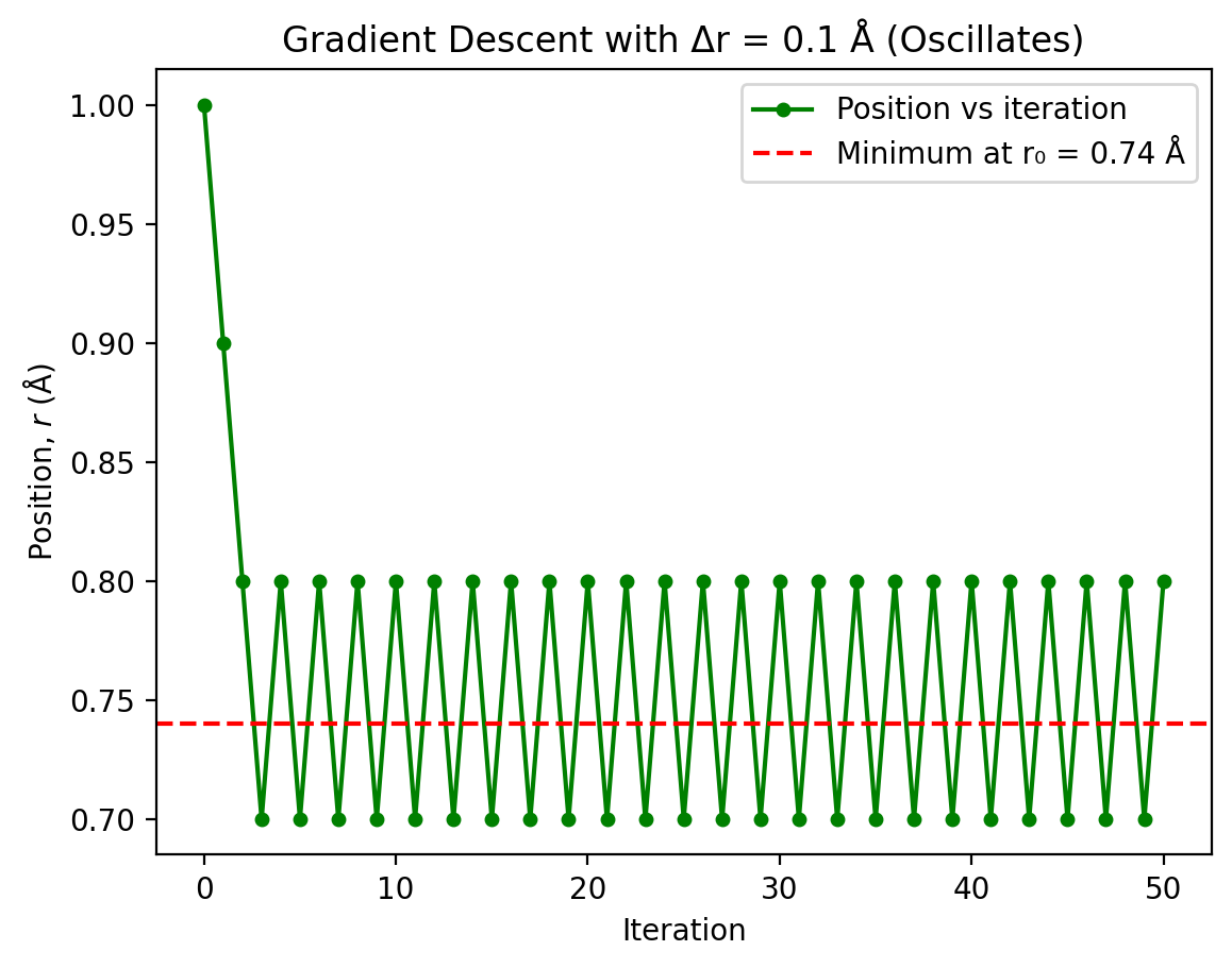
With \(\Delta r = 0.1\) Å, the algorithm fails to converge and instead oscillates around the minimum. Here’s why:
Overshooting: Starting at \(r = 1.0\) Å, the minimum is at \(r_0 = 0.74\) Å, a distance of only 0.26 Å. A step size of 0.1 Å is too large relative to this distance.
The oscillation pattern:
Iteration 0: \(r = 1.0\) Å → gradient positive → step left
Iteration 1: \(r = 0.9\) Å (overshot to the left side of minimum)
Iteration 2: \(r = 0.8\) Å (gradient now negative, step right)
Iteration 3: \(r = 0.9\) Å (back to the right side)
The algorithm bounces back and forth between \(r = 0.8\) Å and \(r = 0.9\) Å
Why no convergence?: The fixed 0.1 Å steps are too large to “land” close enough to the minimum where \(|U'(r)| < 0.001\) eV Å⁻¹. The algorithm perpetually overshoots.
This demonstrates a fundamental limitation of fixed step size gradient descent: the step size must be carefully chosen, and what works for one starting position may not work for another.
Visualizing the oscillation#
Let’s plot both convergence paths to see the difference clearly:
# First, recreate the successful run with small step size for plotting
r_current = 1.0
r_history_small = [r_current]
delta_r_small = 0.01

for iteration in range(26):
    gradient = harmonic_gradient(r_current, k, r_0)
    if abs(gradient) < 0.001:
        break
    r_current = r_current - delta_r_small * np.sign(gradient)
    r_history_small.append(r_current)

# Plot the small step size (converges)
plt.plot(r_history_small, 'o-', markersize=4, linewidth=1.5, label='Position vs iteration')
plt.axhline(r_0, color='r', linestyle='--', label=f'Minimum at r₀ = {r_0} Å')
plt.xlabel('Iteration')
plt.ylabel('Position, $r$ (Å)')
plt.title(f'Gradient Descent with Δr = 0.01 Å (Converges)')
plt.legend()
plt.show()

# Plot the large step size (oscillates)
plt.plot(r_history_large, 'go-', markersize=4,
         label='Position vs iteration')
plt.axhline(r_0, color='r', linestyle='--', label=f'Minimum at r₀ = {r_0} Å')
plt.xlabel('Iteration')
plt.ylabel('Position, $r$ (Å)')
plt.title(f'Gradient Descent with Δr = 0.1 Å (Oscillates)')
plt.legend()
plt.show()
Exercise: Adaptive Step Size Gradient Descent#
The fixed step size method showed us that choosing an appropriate step size is crucial but difficult. An adaptive approach rescales the step size based on the local gradient magnitude:
where \(\alpha\) is the learning rate parameter. This approach naturally takes smaller steps near the minimum (where the gradient is small) and larger steps far from the minimum (where the gradient is large).
Part 1: Learning rate α = 0.01#
Let’s implement adaptive step size gradient descent:
def gradient_descent_adaptive(r_start, alpha, k, r_0, max_iterations=50, threshold=0.001):
    """Perform adaptive step size gradient descent.

    Args:
        r_start (float): Starting position (Å).
        alpha (float): Learning rate.
        k (float): Force constant (eV Å⁻²).
        r_0 (float): Equilibrium bond length (Å).
        max_iterations (int): Maximum number of iterations.
        threshold (float): Convergence threshold for |gradient|.

    Returns:
        tuple: (r_history, gradient_history, converged, num_iterations).
    """
    r_current = r_start
    r_history = [r_current]
    gradient_history = []

    print(f"\nAdaptive gradient descent with α = {alpha}\n")
    print("Iteration | Position (Å) | Gradient (eV Å⁻¹) |     Δr (Å)")
    print("-" * 65)

    converged = False
    for iteration in range(max_iterations):
        # Calculate gradient
        gradient = harmonic_gradient(r_current, k, r_0)
        gradient_history.append(gradient)

        # Calculate step size (adaptive)
        step = -alpha * gradient

        print(f"{iteration:9d} | {r_current:12.6f} | {gradient:17.6f} | {step:9.6f}")

        # Check convergence
        if abs(gradient) < threshold:
            print(f"\nConverged after {iteration} iterations!")
            print(f"Final position: r = {r_current:.6f} Å")
            print(f"Analytical solution: r_0 = {r_0} Å")
            print(f"Error: {abs(r_current - r_0):.6f} Å")
            converged = True
            break

        # Update position
        r_current = r_current + step
        r_history.append(r_current)

    if not converged:
        print(f"\nDid not converge within {max_iterations} iterations.")

    return r_history, gradient_history, converged, iteration

# Run with α = 0.01
r_history_01, grad_history_01, converged_01, iters_01 = gradient_descent_adaptive(
    1.0, 0.01, k, r_0
)
Adaptive gradient descent with α = 0.01

Iteration | Position (Å) | Gradient (eV Å⁻¹) |     Δr (Å)
-----------------------------------------------------------------
        0 |     1.000000 |          9.360000 | -0.093600
        1 |     0.906400 |          5.990400 | -0.059904
        2 |     0.846496 |          3.833856 | -0.038339
        3 |     0.808157 |          2.453668 | -0.024537
        4 |     0.783621 |          1.570347 | -0.015703
        5 |     0.767917 |          1.005022 | -0.010050
        6 |     0.757867 |          0.643214 | -0.006432
        7 |     0.751435 |          0.411657 | -0.004117
        8 |     0.747318 |          0.263461 | -0.002635
        9 |     0.744684 |          0.168615 | -0.001686
       10 |     0.742998 |          0.107913 | -0.001079
       11 |     0.741918 |          0.069065 | -0.000691
       12 |     0.741228 |          0.044201 | -0.000442
       13 |     0.740786 |          0.028289 | -0.000283
       14 |     0.740503 |          0.018105 | -0.000181
       15 |     0.740322 |          0.011587 | -0.000116
       16 |     0.740206 |          0.007416 | -0.000074
       17 |     0.740132 |          0.004746 | -0.000047
       18 |     0.740084 |          0.003037 | -0.000030
       19 |     0.740054 |          0.001944 | -0.000019
       20 |     0.740035 |          0.001244 | -0.000012
       21 |     0.740022 |          0.000796 | -0.000008

Converged after 21 iterations!
Final position: r = 0.740022 Å
Analytical solution: r_0 = 0.74 Å
Error: 0.000022 Å
Explanation:
With \(\alpha = 0.01\), the algorithm converges successfully. Let’s examine how the adaptive step sizes work:
Key observations:
Adaptive step sizes: Notice how the “Δr (Å)” column changes:
Early iterations: When far from the minimum, the gradient is large (e.g., 9.36 eV Å−1 initially), so steps are large (−0.0936 Å)
Later iterations: As we approach the minimum, the gradient decreases, and steps become progressively smaller
Near convergence: Steps become very small as the gradient approaches zero
Natural damping: The step size automatically decreases as we approach the minimum because the gradient magnitude decreases. This prevents oscillation.
Efficiency: The adaptive method allows large initial steps when far from the minimum, then automatically refines with smaller steps near convergence, without needing to manually tune the step size.
Why it works: For the harmonic potential, \(U'(r) = k(r - r_0)\), so the gradient is directly proportional to the distance from the minimum. The adaptive step size therefore automatically scales with this distance.
Part 2: Learning rate α = 0.001#
What happens with a smaller learning rate?
# Run with α = 0.001 (smaller)
r_history_001, grad_history_001, converged_001, iters_001 = gradient_descent_adaptive(
    1.0, 0.001, k, r_0
)
Adaptive gradient descent with α = 0.001

Iteration | Position (Å) | Gradient (eV Å⁻¹) |     Δr (Å)
-----------------------------------------------------------------
        0 |     1.000000 |          9.360000 | -0.009360
        1 |     0.990640 |          9.023040 | -0.009023
        2 |     0.981617 |          8.698211 | -0.008698
        3 |     0.972919 |          8.385075 | -0.008385
        4 |     0.964534 |          8.083212 | -0.008083
        5 |     0.956450 |          7.792217 | -0.007792
        6 |     0.948658 |          7.511697 | -0.007512
        7 |     0.941147 |          7.241276 | -0.007241
        8 |     0.933905 |          6.980590 | -0.006981
        9 |     0.926925 |          6.729289 | -0.006729
       10 |     0.920195 |          6.487034 | -0.006487
       11 |     0.913708 |          6.253501 | -0.006254
       12 |     0.907455 |          6.028375 | -0.006028
       13 |     0.901426 |          5.811353 | -0.005811
       14 |     0.895615 |          5.602145 | -0.005602
       15 |     0.890013 |          5.400468 | -0.005400
       16 |     0.884613 |          5.206051 | -0.005206
       17 |     0.879406 |          5.018633 | -0.005019
       18 |     0.874388 |          4.837962 | -0.004838
       19 |     0.869550 |          4.663795 | -0.004664
       20 |     0.864886 |          4.495899 | -0.004496
       21 |     0.860390 |          4.334046 | -0.004334
       22 |     0.856056 |          4.178021 | -0.004178
       23 |     0.851878 |          4.027612 | -0.004028
       24 |     0.847850 |          3.882618 | -0.003883
       25 |     0.843968 |          3.742844 | -0.003743
       26 |     0.840225 |          3.608101 | -0.003608
       27 |     0.836617 |          3.478210 | -0.003478
       28 |     0.833139 |          3.352994 | -0.003353
       29 |     0.829786 |          3.232286 | -0.003232
       30 |     0.826553 |          3.115924 | -0.003116
       31 |     0.823438 |          3.003751 | -0.003004
       32 |     0.820434 |          2.895616 | -0.002896
       33 |     0.817538 |          2.791374 | -0.002791
       34 |     0.814747 |          2.690884 | -0.002691
       35 |     0.812056 |          2.594012 | -0.002594
       36 |     0.809462 |          2.500628 | -0.002501
       37 |     0.806961 |          2.410605 | -0.002411
       38 |     0.804551 |          2.323823 | -0.002324
       39 |     0.802227 |          2.240166 | -0.002240
       40 |     0.799987 |          2.159520 | -0.002160
       41 |     0.797827 |          2.081777 | -0.002082
       42 |     0.795745 |          2.006833 | -0.002007
       43 |     0.793739 |          1.934587 | -0.001935
       44 |     0.791804 |          1.864942 | -0.001865
       45 |     0.789939 |          1.797804 | -0.001798
       46 |     0.788141 |          1.733083 | -0.001733
       47 |     0.786408 |          1.670692 | -0.001671
       48 |     0.784737 |          1.610547 | -0.001611
       49 |     0.783127 |          1.552568 | -0.001553

Did not converge within 50 iterations.
Explanation:
With \(\alpha = 0.001\), the algorithm does not converge within 50 iterations. After 49 iterations, the gradient is still 1.55 eV Å⁻¹, well above the convergence threshold of 0.001 eV Å⁻¹.
The problem:
Too conservative: With such a small learning rate, each step is very cautious:
Iteration 0: Step is only −0.00936 Å (compared to −0.0936 Å with \(\alpha = 0.01\))
After 49 iterations, we’ve only reached \(r = 0.783\) Å, still 0.043 Å away from the minimum at \(r_0 = 0.74\) Å
Progress is too slow: The gradient decreases very gradually from 9.36 eV Å⁻¹ to 1.55 eV Å⁻¹, but we’re making progress at such a slow rate that we can’t reach convergence.
Many more iterations needed: To converge with this learning rate would require several hundred iterations.
The learning rate is too small: Whilst smaller learning rates are more stable (less likely to diverge), if they’re too small, convergence becomes impractically slow. This learning rate of 0.001 is simply too conservative for efficient optimisation.
Part 3: Learning rate α = 0.1#
What happens with a larger learning rate?
# Run with α = 0.1 (larger)
r_history_1, grad_history_1, converged_1, iters_1 = gradient_descent_adaptive(
    1.0, 0.1, k, r_0, max_iterations=50
)
Adaptive gradient descent with α = 0.1

Iteration | Position (Å) | Gradient (eV Å⁻¹) |     Δr (Å)
-----------------------------------------------------------------
        0 |     1.000000 |          9.360000 | -0.936000
        1 |     0.064000 |        -24.336000 |  2.433600
        2 |     2.497600 |         63.273600 | -6.327360
        3 |    -3.829760 |       -164.511360 | 16.451136
        4 |    12.621376 |        427.729536 | -42.772954
        5 |   -30.151578 |      -1112.096794 | 111.209679
        6 |    81.058102 |       2891.451663 | -289.145166
        7 |  -208.087065 |      -7517.774325 | 751.777432
        8 |   543.690368 |      19546.213244 | -1954.621324
        9 | -1410.930957 |     -50820.154435 | 5082.015444
       10 |  3671.084487 |     132132.401532 | -13213.240153
       11 | -9542.155666 |    -343544.243982 | 34354.424398
       12 | 24812.268732 |     893215.034353 | -89321.503435
       13 | -64509.234703 |   -2322359.089319 | 232235.908932
       14 | 167726.674229 |    6038133.632229 | -603813.363223
       15 | -436086.688994 |  -15699147.443794 | 1569914.744379
       16 | 1133828.055385 |   40817783.353866 | -4081778.335387
       17 | -2947950.280001 | -106126236.720050 | 10612623.672005
       18 | 7664673.392004 |  275928215.472131 | -27592821.547213
       19 | -19928148.155209 | -717413360.227540 | 71741336.022754
       20 | 51813187.867545 | 1865274736.591605 | -186527473.659161
       21 | -134714285.791616 | -4849714315.138174 | 484971431.513817
       22 | 350257145.722201 | 12609257219.359253 | -1260925721.935925
       23 | -910668576.213724 | -32784068770.334057 | 3278406877.033406
       24 | 2367738300.819682 | 85238578802.868561 | -8523857880.286857
       25 | -6156119579.467175 | -221620304887.458282 | 22162030488.745831
       26 | 16005910909.278656 | 576212792707.391602 | -57621279270.739166
       27 | -41615368361.460510 | -1498153261039.218262 | 149815326103.921844
       28 | 108199957742.461334 | 3895198478701.967773 | -389519847870.196777
       29 | -281319890127.735474 | -10127516044625.117188 | 1012751604462.511719
       30 | 731431714334.776245 | 26331541716025.304688 | -2633154171602.530762
       31 | -1901722457267.754395 | -68462008461665.796875 | 6846200846166.580078
       32 | 4944478388898.826172 | 178001222000331.093750 | -17800122200033.109375
       33 | -12855643811134.283203 | -462803177200860.875000 | 46280317720086.093750
       34 | 33424673908951.812500 | 1203288260722238.750000 | -120328826072223.875000
       35 | -86904152163272.062500 | -3128549477877820.500000 | 312854947787782.062500
       36 | 225950795624510.000000 | 8134228642482333.000000 | -813422864248233.375000
       37 | -587472068623723.375000 | -21148994470454068.000000 | 2114899447045407.000000
       38 | 1527427378421683.500000 | 54987385623180576.000000 | -5498738562318058.000000
       39 | -3971311183896374.500000 | -142967202620269504.000000 | 14296720262026952.000000
       40 | 10325409078130578.000000 | 371714726812700800.000000 | -37171472681270080.000000
       41 | -26846063603139504.000000 | -966458289713022208.000000 | 96645828971302224.000000
       42 | 69799765368162720.000000 | 2512791553253857792.000000 | -251279155325385792.000000
       43 | -181479389957223072.000000 | -6533258038460030976.000000 | 653325803846003072.000000
       44 | 471846413888780032.000000 | 16986470899996082176.000000 | -1698647089999608320.000000
       45 | -1226800676110828288.000000 | -44164824339989815296.000000 | 4416482433998981632.000000
       46 | 3189681757888153600.000000 | 114828543283973521408.000000 | -11482854328397352960.000000
       47 | -8293172570509199360.000000 | -298554212538331168768.000000 | 29855421253833117696.000000
       48 | 21562248683323916288.000000 | 776240952599660986368.000000 | -77624095259966095360.000000
       49 | -56061846576642179072.000000 | -2018226476759118512128.000000 | 201822647675911864320.000000

Did not converge within 50 iterations.
Explanation:
With \(\alpha = 0.1\), the algorithm diverges! The position oscillates with increasing amplitude and never converges.
Why this happens:
Overcorrection: The first step is: $\(\Delta r_0 = -\alpha U'(r_0) = -0.1 \times 9.36 = -0.936 \text{ Å}\)\( This moves from \)r = 1.0\( Å to \)r = 0.064\( Å, overshooting the minimum at \)r_0 = 0.74$ Å by a large margin.
Growing oscillations: Each subsequent step overshoots even more dramatically:
The gradient on the far side of the minimum has opposite sign and large magnitude
The large \(\alpha\) amplifies this, causing increasingly wild swings
The position alternates sides but moves further from the minimum each time
Instability criterion: For the harmonic potential with \(U'(r) = k(r - r_0)\), the algorithm is stable when: $\(\alpha < \frac{2}{k}\)\( For our case with \)k = 36.0\( eV Å⁻²: \)\(\alpha < \frac{2}{36} \approx 0.056\)\( Our \)\alpha = 0.1$ exceeds this threshold, causing divergence.
This demonstrates that whilst adaptive step sizes help, the learning rate parameter must still be chosen carefully. Too small and convergence is slow; too large and the algorithm diverges.
Summary: Choosing the learning rate#
Adaptive vs. fixed: Adaptive step sizes (\(r_{i+1} = r_i - \alpha U'(r_i)\)) can outperform fixed step sizes because they automatically adjust based on proximity to the minimum.
The learning rate determines convergence speed: There’s a “sweet spot” for \(\alpha\):
Too small: stable but slow
Just right: fast convergence
Too large: divergence
Problem-specific tuning: The optimal \(\alpha\) depends on the problem (specifically, the curvature \(k\) for harmonic potentials). For different force constants, different learning rates would be optimal.