Exponentials

We may use the term “exponential growth” as a way to describe the rate of a reaction as the temperature increases. In using this phrase, we are describing a very fast rate of increase. We can represent this idea mathematically with one of the simplest exponential equations:

\[ y = a^x \]

where, \(a\) is a constant, \(x\) is the controlled variable (in the above case, temperature), and \(y\) is the observed variable (in the above case, rate of reaction).

Show code cell source

Hide code cell source

import numpy as np
import matplotlib.pyplot as plt

x = np.linspace(-4, 6, 100)
y = 2 ** x

fig, ax = plt.subplots()
ax.plot(x, y)
ax.set_xlabel('x')
ax.set_ylabel('y')
plt.show()

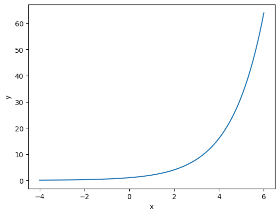
Above, we have the graph of \(y=2^x\) and we can see the graph increases at a very fast rate, which is what we would expect with exponential growh. Other mathematical things to note are:

• The graph passes through the point (0, 1), as any variable raised to the power of 0 is equal to 1.

• The values of \(y\) are small and positive when \(x\) is negative.

• The values of \(y\) are large and positive when \(x\) is postive.

The Exponential Function

So far, we have used the word exponential to describe equations in the form \(y=a^x\). However, the word is usually reserved to describe a special type of function. It is quite likely we will have see the symbol π before, and know it represented the irrational number 3.14159265…. In this section, we will be working with the number:

\[ e = 2.7182818\ldots \]

Note

Another notation for \(e^x\) is \(\exp(x)\). They mean the same thing.

Like π, e is another number that goes on forever! when we refer to the exponential function, we mean \(y=e^x\). This can be seen as a special case of the previous section, when the constant is \(a=e\), in the equation \(y=a^x\). When we refer to \(e^x\), we say “e to the x”.

---

There are two ways to access the value e in Python.

import numpy as np

np.e

2.718281828459045

np.exp(1)

2.718281828459045

---

Arrhenius Equation

The Arrhenius equation below describes the exponential relationship between the rate of a reaction \(k\) and the temperature \(T\).

\[ k = A\exp{\left(\frac{-E_a}{RT}\right)} \]

where \(R\), \(E_a\) and \(A\) are all constants. Support for a reaction that the activation energy is \(E_a=52.0\;\textrm{kJ mol}^{-1}\), the gas constant \(R = 8.314\;\textrm{JK}^{-1}\textrm{mol}^{-1}\) and \(A = 1.00\). What is the rate of the reaction \(k\), when the temperature \(T=241\;\textrm{K}\)?

Solution: We substitute our given values from the question into the Arrhenius equation.

\[\begin{split} \begin{aligned} k & = A\exp{\left(\frac{-E_a}{RT}\right)} \\ k & = 1 \times \exp{\left(\frac{-52\times10^{3}}{8.314 \times 241}\right)} \\ k & = \exp(-25.9509\ldots) \\ k & = 5.3663\ldots \times 10^{-12} \\ k & = 5.37 \times 10^{-12} \textrm{(to 3 s.f.)} \end{aligned} \end{split}\]

---

Python is great for doing computations such as these.

Python Note

In this code cell, we import the constant \(R\) from the scipy.constants library.

from scipy.constants import R

E_a = 52e3
T = 241 
A = 1

k = A * np.exp(-E_a / (R * T))
k

5.3663046790901465e-12

---

Exponential Graphs

Exponential graphs follow two general shapes, called growth and decay, which are shown below.

Show code cell source

Hide code cell source

x1 = np.linspace(-6, 2, 100)
y1 = np.exp(x1)
x2 = np.linspace(-2, 6, 100)
y2 = np.exp(-x2)

fig, (ax1, ax2) = plt.subplots(1, 2, figsize=(10, 4))
ax1.plot(x1, y1)
ax1.set_xlabel('x')
ax1.set_ylabel('y = exp(x)')
ax2.plot(x2, y2, color='orange')
ax2.set_xlabel('x')
ax2.set_ylabel('y = exp(-x)')
plt.tight_layout()
plt.show()

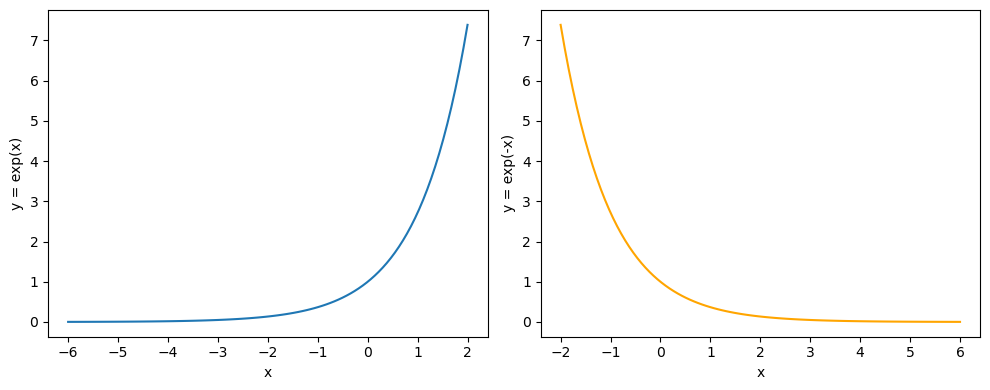
• On the left exponential growth, which is represented by the equation \(y=e^x\), note that the graph gets steeper from left to right.

• On the right exponential growth, which is represented by the equation \(y=e^{-x}\), note that the graph gets shallowed from left to right.

Alegbraic Rules for Exponentials

We use very similar rules as the ones we had for powers. The only difference is that the base is now a constant and the power is a variable.

Note

Here, we have that \(x\) and \(y\) are variables and \(a\) is a constant, for example \(a=e\) or \(a=3\). In order to use the rules, \(a\) must be the same for all terms. For example, we cannot simplify \(e^x \times 3^x \times 4^x\).

1. \(a^x \times a^y = a^{x+y}\)

2. \(\frac{a^x}{a^y} = a^{x-y}\)

3. \((a^x)^y = a^{x\times y}\)

Example

Simplify the following equations:

1. \(y = 3^x \times 3^{2x}\)

2. \(y = \frac{2^x}{4}\)

3. \(y = \left(e^{-x+1}\right)^x\)

Solution:

1. Since the bases ar ehte same, we use the first rule.

   \[ y = 3^x \times 3^{2x} = 3^{x+2x} = 3^{3x} \]

2. The first thing we notice is that \(4\) can be written as \(2^2\) so:

   \[ y = \frac{2^x}{2^2} \]

   Now that we have powers to the same base, we can apply the rules. Using the second rule, we have:

   \[ y = 2^{x-2} \]

3. Using the third rule, we get that:

   \[ y = \left(e^{-x+1}\right)^x = e^{-x^2+x} \]

---

The sympy package is aware of these rules.

from sympy import symbols

x = symbols('x')

3 ** x * 3 ** (2 * x)

\[\displaystyle 3^{3 x}\]

from sympy import simplify

simplify(2 ** x / (2 ** 2))

\[\displaystyle 2^{x - 2}\]

Unfortunately, the final example does not work with sympy.

---