Introduction to Vectors#
When describing some quantities, just a number and units aren’t enough. Say we are navigating a ship across the ocean and we are told that the port is 5 km away, we don’t know in which direction we have to sail. 5 km due east would give us all the information we need. This is an example of a vector, a quantity that has magnitude and direction.
Some chemistry related vector quantities are velocity, force, acceleration, linear and angular momentum and electric and magnetic fields.
Quantities that have just a magnitude are scalars. Examples of these are temperature, mass, and speed.
Vectors in 2-D Space#
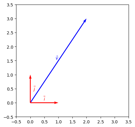
A vector in 2-D space can be written as a combination of 2 base vctors, \(\vec{i}\) being a horizontal vector (in the x-direction) and \(\vec{j}\) being in the vertical vector (in the y-direction). They are both unit vectors, meaning that their length (magnitude) is 1. For an example, the vector \(\vec{v} = 2\vec{i} + 3\vec{j}\) is shown below:
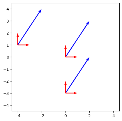
The vector \(\vec{v}\) above also describes all vector at move \(2\vec{i}\) units and \(3\vec{j}\) units, they don’t have to start at the origin. All the vectors in the graph below are exactly the same.
fig, ax = plt.subplots()

for x, y in [[0, 0], [-4, 1], [0, -3]]:
    ax.scatter([x, v[0]], [y, v[1]], marker='')
    ax.quiver(x, y, v[0], v[1], angles='xy', scale_units='xy', scale=1, color='b')
    ax.quiver(x, y, 0, 1, angles='xy', scale_units='xy', scale=1, color='r')
    ax.quiver(x, y, 1, 0, angles='xy', scale_units='xy', scale=1, color='r')
ax.set_aspect('equal')
ax.set_xlim(-4.5, 4.5)
ax.set_ylim(-4.5, 4.5)

plt.show()
Writing a general 2-D vector \(\vec{u}\) as a combination of the unit vectors would give:
where \(a\) and \(b\) are real numbers.
In Python, we can represent any vector using a NumPy array. For example, the vector \(\vec{v}\) above can be represented as:
import numpy as np

v = np.array([2, 3])
print(v)
[2 3]
We will use this vector in some examples later.
Vectors in 3-D Space#
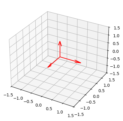
Any vector in 3-D space can be written as a combination of 3 base vectors; \(\vec{i}\), \(\vec{j}\), \(\vec{k}\) each being the unit vector in the x-, y-, and z-dimensions. Below is a plot of the 3 axes with their repective unit vectors:
Writing a general vector \(\vec{v}\) as a combination of the unit vectors would give:
where \(a\), \(b\), and \(c\) are real numbers.
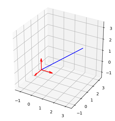
To extend a NumPy array to 3-D simply involves adding another value, i.e.,
u = np.array([2, 3, 1])
print(u)
[2 3 1]
We can visualise this in a 3-D plot with matplotlib.
ax = plt.figure().add_subplot(projection='3d')

ax.quiver(0, 0, 0, 1, 0, 0, length=1, color='r')
ax.quiver(0, 0, 0, 0, -1, 0, length=1, color='r')
ax.quiver(0, 0, 0, 0, 0, 1, length=1, color='r')
ax.plot([0, u[0]], [0, u[1]], [0, u[2]], color='b')

ax.set_xlim3d(-1.5, 3.5)
ax.set_ylim3d(-1.5, 3.5)
ax.set_zlim3d(-1.5, 3.5)

ax.set_aspect('equal')

plt.show()
Representations of Vectors#
A vector \(\vec{v}\) can be written in the following forms:
Unit vector notation:
\[ \vec{v} = a\vec{i} + b\vec{j} + c\vec{k} \]The vector is displayed as the clear sum of its base vectors. In 3-D space, those are the \(\vec{i}\), \(\vec{j}\), and \(\vec{k}\) vectors.
Ordered set notation:
\[ \vec{v} = (a, b, c) \]The vector is in the same form as unit vector notation (\(a\), \(b\), and \(c\) are the same numbers) but it is more compact notation.
Column notation:
\[\begin{split} \vec{v} = \begin{pmatrix} a \\ b \\ c \end{pmatrix} \end{split}\]This is identical to ordered set notation apart from it being vertical. This form makes some calculations easier to visualise, such as the dot product.
For example, the 2-D vector \(\vec{u}\) shown below can be written as \(\vec{u} = 4\vec{i} + 3\vec{j}\) or \(\vec{u} = (4, 3)\) or \(\vec{u} = \begin{pmatrix} 4 \\ 3 \end{pmatrix}\).
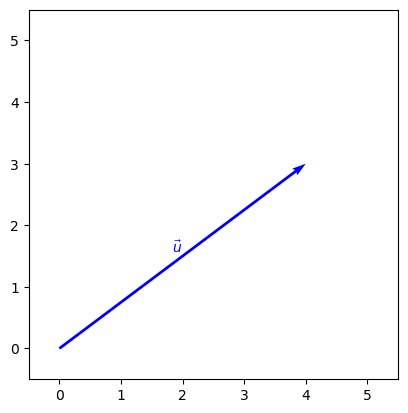
Magnitude of Vectors#
If we know the lengths of each of the component vectors, we can find the length (or magnitude), \(|\vec{v}|\), of the vector using Pythagoras theorem. For a 3-D vector \(\vec{v} = a\vec{i} + b\vec{j} + c\vec{k}\):
For vector \(\vec{u} = 4\vec{i} + 3\vec{j}\) above, we can calculate the magnitude \(|\vec{u}| = \sqrt{4^2+3^2} = \sqrt{16+9} + \sqrt{25} = 5\)
Example
Find the magnitude of the following vectors:
\((2, 6, 3)\)
\(\vec{i} + 7\vec{j} + 4\vec{k}\)
\(\begin{pmatrix} \sqrt{2} \\ \sqrt{2} \\ 0 \end{pmatrix}\)
Solution:
\(|(2, 6, 3)| = \sqrt{2^2 + 6^2 + 3^2} = \sqrt{4+36+9} = \sqrt{49} = 7\)
\(| \vec{i} + 7\vec{j} + 4\vec{k} | = \sqrt{1^2 + 7^2 + 4^2} = \sqrt{1 + 49 + 16} = \sqrt{66}\)
\(\left| \begin{pmatrix} \sqrt{2} \\ \sqrt{2} \\ 0 \end{pmatrix} \right| = \sqrt{(\sqrt{2})^2 + (\sqrt{2})^2} = \sqrt{2+2} = \sqrt{4} = 2\)
In Python, we can obtain the magnitude by squaring all the values, summing them, and finding the square root.
np.sqrt(np.sum(np.array([2, 6, 3]) ** 2))
7.0
Or it is possible to use the np.linalg.norm function.
np.linalg.norm(np.array([1, 7, 4]))
8.12403840463596
To show that these are equivalent.
v = np.array([np.sqrt(2), np.sqrt(2), 0])

np.sqrt(np.sum(v ** 2)), np.linalg.norm(v)
(2.0, 2.0)
Helium Velocity
A helium atom is moving with a velocity \(\vec{v}\) of \(20\vec{i} - 15\vec{j}\) ms-1. What is the speed of the atom?
Solution: Since speed is the magnitude of velocity, we take the magnitude of the velocity vector. This gives:
Therefore, the particles speed is 25 ms-1.
And with NumPy, this looks like:
v = np.array([20, -15])
np.linalg.norm(v)
25.0