Differentiating Polynomials

A polynomial is an equation in the form:

\[ a_n x_n + a_{n-1}x_{n-1} + \ldots + a_2x^2 + a_1x^1 + a_0 \]

where

• \(a_n, \ldots, a_2, a_1, a_0\) are the constant coefficients.

• \(x^n, x^{n-1}, \ldots, x^2\) are powers of a variable \(x\).

A rather simple example of a polynomial is the quadratic \(x^2+3x+1\).

Differentiation finds the gradient of a curve at a given point. Suppose we want to find the gradient of a function that is a polynomial, such as \(y = x^3+1\). How do we find this differential?

As differentiation may be new to many readers, we will begin slowly and first explain how to differentiate the individual terms of a polynomial, for example \(x^2\), before moving on in the section on differentiating a sum to help us differentiate polynomial sums such as \(4x^3+1\).

The general rule is as follows:

\[ \textrm{If }y=x^n\textrm{, then }\frac{dy}{dx} = nx^{n-1} \]

The main points we should note are that:

• If \(y=1\), then \(\frac{dy}{dx} = 0\) (since \(x^0=1\), so \(n=0\) here). In fact, the same can be applied to any constant, not just 1. So:

  \[ \textrm{If }y=c\textrm{ for any constant }c\textrm{, then }\frac{dy}{dx} = 0 \]

• If we have \(y=x\), then this is the same as \(y=x^1\), so we have \(\frac{dy}{dx}=1\times x^{1-1} = 1\).

• If we have \(y=x^2\), then we have \(\frac{dy}{dx} = 2\times x^{2-1} = 2x\).

We have only considered examples of polynomials up to the power of 2. The next example shows that we can apply this rule to polynomials of higher powers.

Example

Differentiate \(y=x^5\).

Solution: From above, we know if \(y=x^n\), then \(\frac{dy}{dx} = nx^{n-1}\). So in this example, we have that \(n=5\). This gives the following answer:

\[ \frac{dy}{dx} = 5x^{5-1} = 5x^4 \]

---

The sympy library that we met previously is also capable of symbolic differentiation.

from sympy import symbols, diff

x = symbols('x')

diff(x ** 5)

\[\displaystyle 5 x^{4}\]

---

We can also differentiate using this rule when $x$ is raised to a negative power, as shown in the next example.

Example

Differentiate \(y=x^{-1}\).

Solution: From above, we know if \(y=x^n\), then \(\frac{dy}{dx} = nx^{n-1}\). So in this example, we have that \(n=-1\). This gives the following answer:

\[ \frac{dy}{dx} = -1 \times x^{-1-1} = -x^{-2} \]

---

Note

Recall that \(x^{-2} \equiv \frac{1}{x^2}\).

diff(x ** -1)

\[\displaystyle - \frac{1}{x^{2}}\]

---

We can differentiate using this rule when \(x\) is raised to a fractional power, as shown in the next example.

Example

Differentiate \(y = x^{\frac{1}{2}}\).

Solution: So using the rule if \(y = x^n\), when \(\frac{dy}{dx} = nx^{n-1}\), we have \(n=\frac{1}{2}\). This gives the answer:

\[ \frac{dy}{dx} = \frac{1}{2}\times x^{\frac{1}{2} - 1} = \frac{x^{-1}{2}}{2} \]

---

diff(x ** (1/2))

\[\displaystyle \frac{0.5}{x^{0.5}}\]

It is an exercise for the reader to show the above Python result is equivalent to the mathematical result above.

---

So far, we have only considered polynomials, which has a coefficient of 1. But how do we differentiate \(y=4x^2\), where the coefficient is equal to 4? When we have a coefficient, denotated \(a\), we have the rule:

Note

The first rule is just a special case of this rule, when \(a=1\).

\[ \textrm{If }y = ax^n\textrm{ then }\frac{dy}{dx} = a\times n \times x ^{n-1} \]

So going back to \(y=4x^2\), we can see that the coefficient \(a=4\) and \(x\) is raised to the power \(n=2\). So using the rule if \(y=ax^n\), then \(\frac{dy}{dx}= a\times n\times x^{n-1}\). We have:

\[ \frac{dy}{dx} = 4\times 2\times x^{2-1} = 8x^1 = 8x \]

Important

When differentiating any function \(f(x)\), multipled by some constant \(a\), finding \(\frac{d}{dx}[af(x)]\), we can take the constant \(a\) out of the derivative so:

\[ \frac{d}{dx}[df(x)] = a\frac{d}{dx}[f(x)] \]

For example, \(\frac{d}{dx}(2x^3) = 2\times \frac{d}{dx}(x^3) = 2\times 3x^2 = 6x^2\).

Example

Differentiate \(y=4x^{-\frac{1}{2}}\)

Solution: This example combines everything we have looked at so far. So using the rule:

\[ \textrm{If }y=ax^n\textrm{ then }\frac{dy}{dx}=a\times n\times x^{n-1} \]

We have \(a=4\) and \(n=-\frac{1}{2}\). This gives the answer:

\[ \frac{dy}{dx} = 4\times -\frac{1}{2}\times x^{-\frac{1}{2} - 1} = -2x^{-\frac{3}{2}} \]

---

diff(4 * x ** -0.5)

\[\displaystyle - \frac{2.0}{x^{1.5}}\]

---

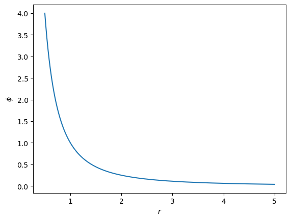
Coulomb’s Law

Coulomb’s Law starts that the magnitude of the attractive force \(\phi\) between two charges decays accounding to the inverse swquare of the intervening distance \(r\):

\[ \phi = \frac{1}{r^2} \]

Supporse we plot a graph of \(\phi\) on the y-axis against \(r\) on the x-axis, what is the gradient.

Solution: To find the gradient, we find the derviative with respect to \(r\), denoted \(\frac{d\phi}{dr}\) of:

\[ \phi = \frac{1}{r^2} = r^{-2} \]

All the examples so far have only contained \(x\) and \(y\), however in this question, we have the variables \(\phi\) and \(r\). We know \(y=x^n\) then \(\frac{dy}{dx}=nx^{n-1}\), so with \(y\) as \(\phi\) and \(x\) and \(r\) and \(n=-2\). We have:

\[ \frac{d\phi}{dr} = -2 \times r^{-2-1} = -2 r^{-3} = -\frac{2}{r^3} \]

---

In Python, we will start by plotting the relationship.

import numpy as np
import matplotlib.pyplot as plt

r = np.linspace(0.5, 5, 1000)
phi = 1 / (r ** 2)

plt.plot(r, phi)
plt.xlabel('$r$')
plt.ylabel('$\phi$')
plt.show()

We can then use sympy to find the gradient at any point, \(r\).

r = symbols('r')

diff(1 / (r ** 2))

\[\displaystyle - \frac{2}{r^{3}}\]

The equation above tells us that \(\frac{d\phi}{dr}\) will be negative for all positive \(r\). We can see this in the plot above, the slope of the line is always going down.

---