Stationary Points

Stationary points occur when we have \(\frac{dy}{dx} = 0\); this represents when the gradient of a curve is horizontal, we have three types of stationary point:

1. Local maximum

Show code cell source

Hide code cell source

import numpy as np
import matplotlib.pyplot as plt

x = np.linspace(-2, 2, 100)
y = -(x ** 2) + 1.5

plt.plot(x, y)
plt.axhline(1.5, xmin=0.25, xmax=0.75, color='r', linestyle='--')
plt.show()

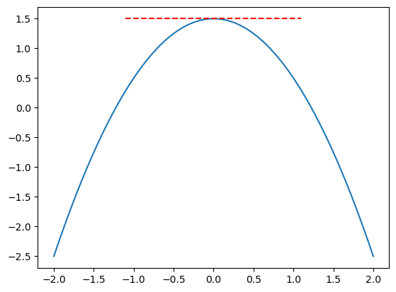
We can see that when we pass through the maximum, the gradient goes from being positive (\(\frac{dy}{dx} > 0\)) to being negative (\(\frac{dy}{dx} < 0\)).

2. Local minimum

Show code cell source

Hide code cell source

y = x ** 2 - 1.5

plt.plot(x, y)
plt.axhline(-1.5, xmin=0.25, xmax=0.75, color='r', linestyle='--')
plt.show()

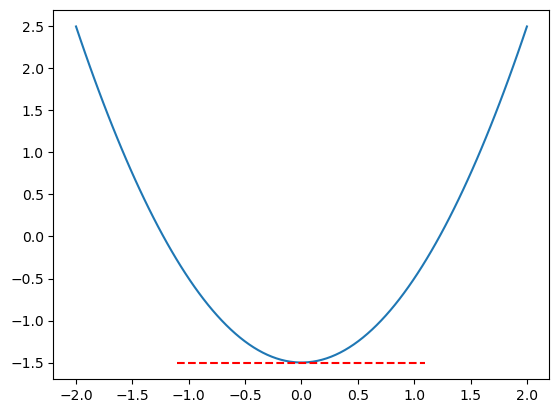
We can see that when we pass through a minimum, the gradient goes from being negative (\(\frac{dy}{dx} < 0\)) to being positive (\(\frac{dy}{dx} > 0\)).

3. Point of inflection

Show code cell source

Hide code cell source

x = np.linspace(-1, 1, 100)
y = x ** 3 + 0.5

plt.plot(x, y)
plt.axhline(0.5, xmin=0.25, xmax=0.75, color='r', linestyle='--')
plt.show()

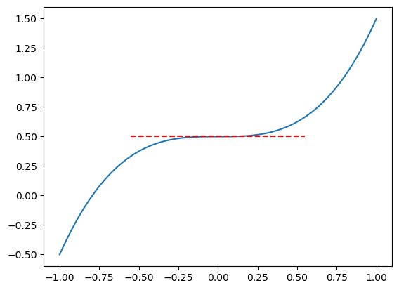
Finally, when we pass through a point of inflection, we should note that the gradient remains of the same sign (so either positive or negative on both sides).

Example

Find the stationary point of \(y=x^2\).

Solution: From the graph of \(y=x^2\), we can see that there is a minimum at \(x=0\), however, we need to find this algebraically.

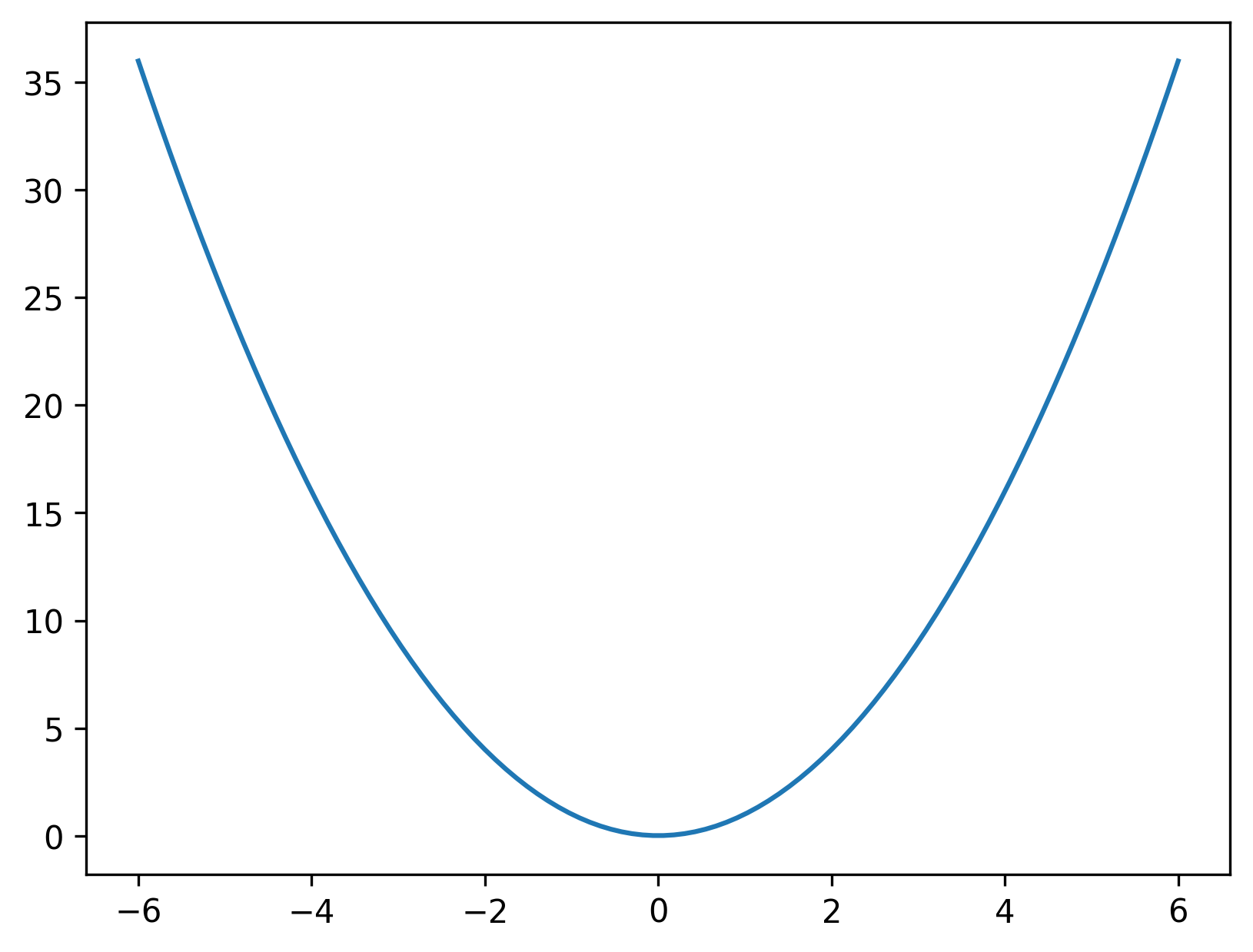
First, we nee to find when \(\frac{dy}{dx} = 0\). Now \(\frac{dy}{dx} = 2x\) and therefore, \(\frac{dy}{dx}=0\) when \(x=0\).

So we know we have a stationary point at \(x=0\). In the next section, we will discuss how to decide whether this is a maximum, minimum, or point of inflection.

Classifying Stationary Points

We now need to introduce the second derivative, denoted:

\[ \frac{d^2y}{dx^2}\;\;\;\text{or}\;\;\;f''(x) \]

This means that we differentiate a function twice, so for example, if we have \(y=x^3\), we would first find:

\[ \frac{dy}{dx} = 3x^2 \]

which we would then differentiate again to find:

\[ \frac{d^2y}{dx^2} = 6x. \]

---

sympy can easily compute the second, or higher order, derivative.

from sympy import symbols, diff

x = symbols('x')

diff(diff(x ** 3))

\[\displaystyle 6 x\]

---

First Test

The second derivative is used to decide whether a stationary point is a maximum or a minimum. If we have a value of \(x\) of a stationary point, then we substitute that value into the second derivative, if:

• \(\frac{d^2y}{dx^2} > 0\), so positive, we have a minimum.

• \(\frac{d^2y}{dx^2} <> 0\), so negative, we have a maximum.

Unfortunately, this test fails if we find that \(\frac{d^2y}{dx^2} = 0\). In this case, we could have a maximum, minimum, or point of inflection and we must carry out the following further test in order to decide.

Second Test

First, first two \(x\) values, just to the left and right of the stationary point and calculate \(f'(x)\) for each. Let us denote the \(x\) value just to the left as \(x_L\) and the one to the right as \(x_R\), then if:

• \(f'(x_L) > 0\) and \(f'(x_R) < 0\), we have a minimum.

• \(f'(x_L) < 0\) and \(f'(x_R) > 0\), we have a maximum.

• \(f'(x_L)\) and \(f'(x_R)\) have the same sign (so both are either positive of negative), then we have a point of inflection.

Example

class: example Find and classify the stationary points of \(y=\frac{x^4}{4} - \frac{x^2}{2}\).

Solution: First, we find when \(\frac{dy}{dx} = 0\) to find where the stationary points are.

\[\begin{split} \begin{aligned} \frac{dy}{dx} & = x^3 - x = 0 \\ & = x(x^2 - 1) = 0 \\ & x(x-1)(x+1) = 0 \end{aligned} \end{split}\]

Therefore, we have stationary points at \(x=0\), \(x=1\), and \(x=-1\) to classify them, we first must find the second derivative:

\[ \frac{d^2y}{dx^2} = 3x^2 - 1 \]

Now we substitute our \(x\)-values for the location of the stationary point into \(\frac{d^2y}{dx^2}\):

• When \(x=0\), we have \(\frac{d^2y}{dx^2} = -1, hence \)\frac{d^2y}{dx^2} < 0$ (negative), so this is a maximum.

• When \(x=1\), we have \(\frac{d^2y}{dx^2} = 2, hence \)\frac{d^2y}{dx^2} > 0$ (positive), so this is a minimum.

• When \(x=-1\), we have \(\frac{d^2y}{dx^2} = 2, hence \)\frac{d^2y}{dx^2} > 0$ (positive), so this is a minimum.

---

Let’s look at doing this in Python. In addition to being able to perform differentiation, sympy can help us find the stationary points.

from sympy import stationary_points

y = x ** 4 / 4 - x ** 2 / 2
sp = stationary_points(y, x)
sp

\[\displaystyle \left\{-1, 0, 1\right\}\]

We then find the second derivative.

second = diff(diff(y))
second

\[\displaystyle 3 x^{2} - 1\]

And we iterate through the stationary points to find the value of \(\frac{d^2y}{dx^2}\) and perform the first test.

Python Note

A sympy Set-type object can be converted to a standard Python list but passing it to the list() function.

for point in list(sp):
    value = second.evalf(subs={x: point})
    print(f'x = {point}; d^2y/dx^2 = {value:.0f}')

x = -1; d^2y/dx^2 = 2
x = 0; d^2y/dx^2 = -1
x = 1; d^2y/dx^2 = 2

This matches the findings above.

---

Example

Find and classify the stationary points of \(y = x^3\).

Solution: First, we find when \(\frac{dy}{dx} = 0\) to find where the stationary points are.

\[\begin{split} \begin{aligned} \frac{dy}{dx} & = 3x^2 = 0 \\ & = x = 0 \end{aligned} \end{split}\]

Now, when \(x=0\), we have \(\frac{d^2y}{dx^2} = 0\), hence our test has failed and we must carried out the further test.

We need to pick \(x\) values close to either side of the stationary point at \(x=0\). So a \(x\) value just to the left would be \(x_L = -0.5\) and one just to the right would be \(x_R = 0.5\).

Since \(\frac{dy}{dx} = 3x^2\), we have that:

• \(f'(x_L) = 3(x_L)^2 = 3 \times -0.5 ^ 2 = 0.75 > 0\)

• \(f'(x_R) = 3(x_R)^2 = 3 \times 0.5 ^ 2 = 0.75 > 0\)

Both \(f'(x_L) > 0\) and \(f'(x_R) > 0\) are positive, so are of the same sign. Hence the stationary point at \(x=0\) is a point of inflection.

---

We could check this using sympy. However, here we will use a graphical assessment by plotting the function, \(x^3\).

Show code cell source

Hide code cell source

x = np.linspace(-1, 1, 100)
y = x ** 3

plt.plot(x, y)
plt.xlabel('$x$')
plt.ylabel('$y$')
plt.show()

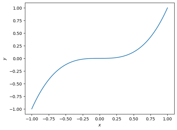
The point of inflection is clear from the graph.

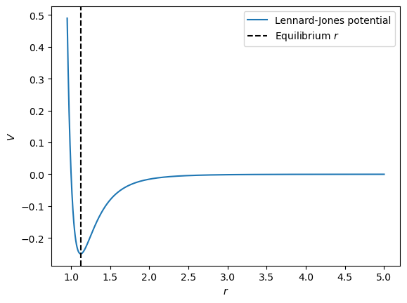
Lennard-Jones Potential

The LennardJones potential describes the potential energy \(v\) between two helium atoms, separated by a distance \(r\). The equation and graph of this function are shown below:

\[ V(R) = \frac{A}{r^{12}} - \frac{B}{r^6} \]

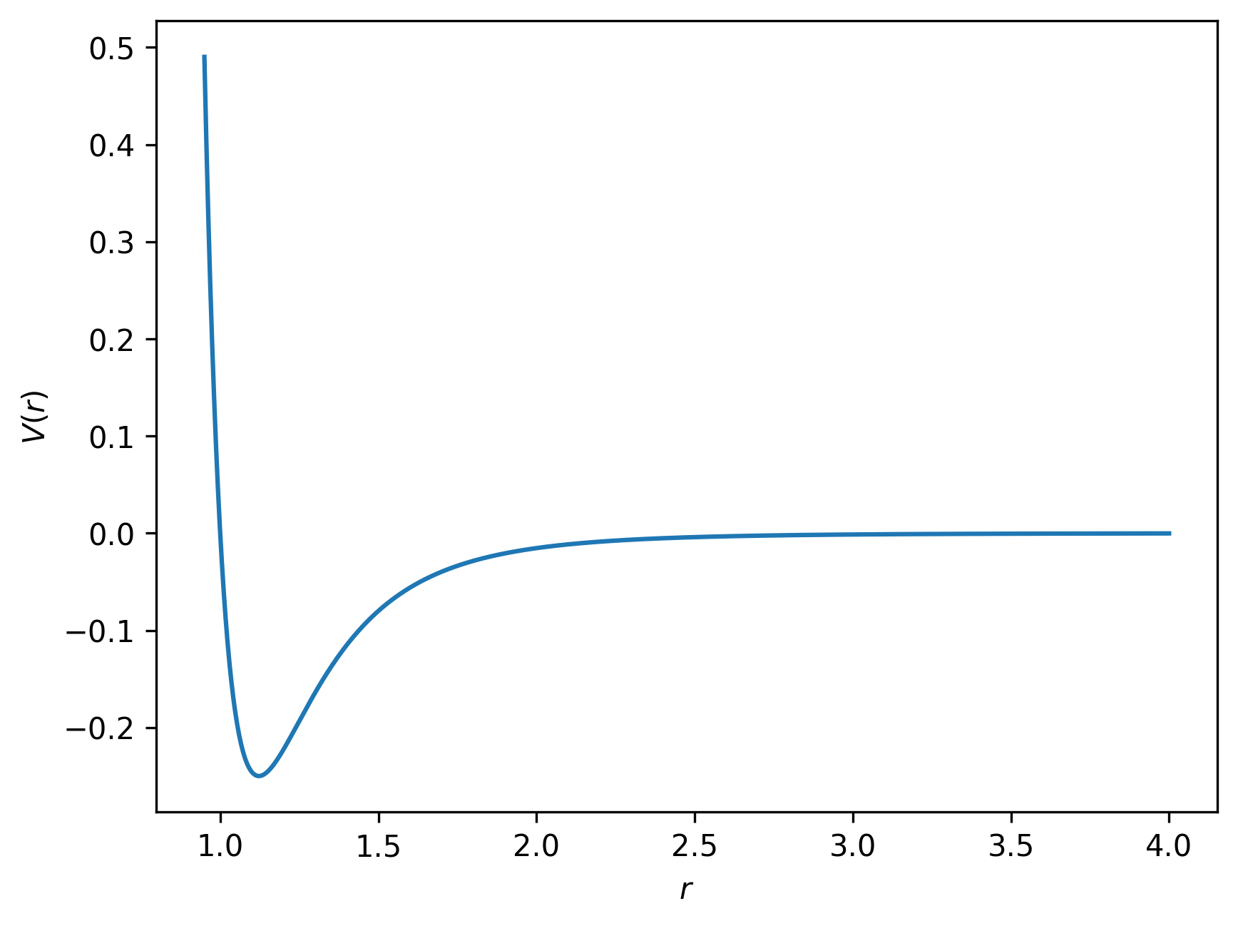
where \(A\) and \(B\) are constants. The two particles are at their equilibrium separation when the potential is at a minimum (\(V\) is at a minimum). By differentiating this equation, with respect to \(r\), find the equilibrium separation.

Solution: To find the minimum \(V\), we need to differentiate it and then set it equal to zero (find \(\frac{dV}{dr} = 0\)). Then that value of \(r\) will be where the potential is a minimum. Differentiating \(V\) with respect to \(r\) gives:

\[ \frac{dV}{dr} = \frac{-12A}{r^{13}} + \frac{6B}{r^7} \]

We need to find when \(\frac{dV}{dr} = 0\), we need to solve the equation:

• Add \(\frac{-12A}{r^{13}}\) to both sides: \(\frac{6B}{r^7} = \frac{12A}{r^{13}}\)

• Multiply each side by \(r^{13}\) and divide by \(6B\): \(\frac{r^{13}}{r^7} = \frac{12A}{6B}\)

• Simplify both of the fractions: \(r^6 = \frac{2A}{B}\)

• That the 6th root of both sides: \(r = \left(\frac{2A}{B}\right)^{\frac{1}{6}}\)

Hence the equilibrium separation is \(r = \left(\frac{2A}{B}\right)^{\frac{1}{6}}\).

---

We can see this in Python, then compute and plot the equilibrium distance for any \(A\) and \(B\).

A, B, r = symbols('A B r')

V = A / r ** 12 - B / r ** 6

first = stationary_points(V, r)
first

\[\displaystyle \left(\left(-\infty, 0\right) \cup \left(0, \infty\right)\right) \cap \left\{- \sqrt[6]{2} \sqrt[6]{\frac{A}{B}}, \sqrt[6]{2} \sqrt[6]{\frac{A}{B}}\right\}\]

The notation above is slightly confusing, but all it says that there are two stationary points, one where \(r\) is between 0 and positive infinity and another between negative infinity and 0. We are interested in the former as we can’t have a distance between atoms of less than 0. We will evaluate this algebra for \(A=1\) and \(B=1\) and convert the results to a Numpy array.

r_equil = np.array(list(first.evalf(subs={A: 1, B: 1})))
r_equil

array([-1.12246204830937, 1.12246204830937], dtype=object)

You will notice there are two values of the equilibrium \(r\). We are only interested in the one that is greater than 0, as outlined above.

r_equil = r_equil[r_equil > 0]
r_equil

array([1.12246204830937], dtype=object)

We can now plot the Lennard-Jones potential, and add a dashed line to show the equilibrium \(r\) position.

r = np.linspace(0.95, 5, 1000)
V = 1 / r ** 12 - 1 / r ** 6

plt.plot(r, V, label='Lennard-Jones potential')
plt.axvline(r_equil, linestyle='--', color='k', label='Equilibrium $r$')
plt.xlabel('$r$')
plt.ylabel('$V$')
plt.legend()
plt.show()

---