Introduction to Integration#
Integration is the opposite of differentiation, so it helps us find the answer to the question:
Suppose we have \(\frac{dy}{dx} = 2x\), then what is \(y\)?
From the previous section, we know the answer is \(x^2+C\), where \(C\) is a constant. So we would say that \(2x\) integrated is \(x^2+C\).
Graphically, we know differentiation gives us the gradient of a curve. Integration finds the area beneath a curve.
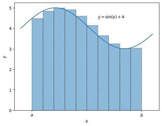
Suppose we wish to find the area under the curve between the \(x\) values \(a\) and \(b\) shaded in the graph above. Then we could find an approximate answer by creating the dashed retectangles above and summing their area.
We can use Python to perform this computation, it is known as a Reimann sum. To find a Reimann sum, the equation, \(y=\sin{(x)} + 4\) is computed for each of the rectangles above.
y_rect = np.sin(x_rect) + 4
y_rect
array([4.47942554, 4.84147098, 4.99749499, 4.90929743, 4.59847214,
       4.14112001, 3.64921677, 3.2431975 , 3.02246988, 3.04107573])
Next, we compute the area for each of the rectangle.
areas = y_rect * (x_rect[1] - x_rect[0])
areas
array([2.23971277, 2.42073549, 2.49874749, 2.45464871, 2.29923607,
       2.07056   , 1.82460839, 1.62159875, 1.51123494, 1.52053786])
And finally a summation is found.
np.sum(areas)
20.461620486839937
So an estimate of the integral of \(y=\sin{(x)} + 4\) is approximately 20.46 (to 2 s.f.).
We can see that this coarse representation would not give a perfect answer, however, the smaller the width of the rectangles, the better the estimation of the integral would be.
So if we could use rectangles of an infinitely small width we would find an answer with minimal error. This is what integration does. It creates an infinite number of rectangles under the curve all with an infinitely small width and sums their area to find the area under the curve.
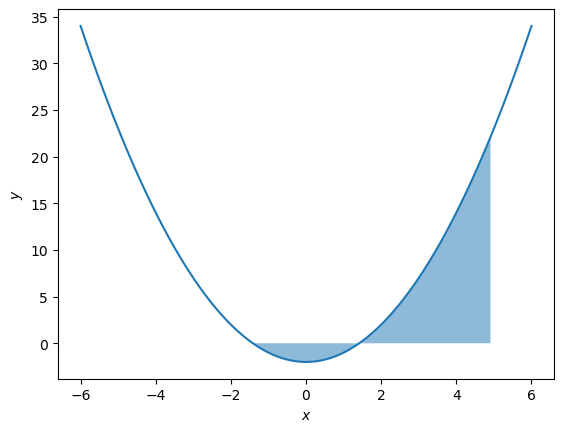
So integration could be used to find the area shaded on the graph of \(y = x^2-2\) above. Note that when the curve is below the \(x\)-axis, integration finds the area bounded between the curve and the \(x\)-axis.
Notation#
We use the fact that \(2x\) integrated is \(x^2+C\) to help introduce the following notation for integration. If we want to integrate \(2x\), we write this as:
The \(\int\) tells us we need to integrate.
The \(dx\) tells us to integrate with respect to \(x\). So we could write \(\int 2z\;dz = z^2 + C\), but in this case we have integrated with respect to \(z\).
We call \(\int 2x\;dx = x^2+C\) the integral.
Another notation often used is the following, if we have the function \(f(x)\), then we write this integrated as \(F(x)\). So if \(f(x) = 2x\), then \(F(x) = x^2+C\).
Integration finds the area under the curve. So if we want to find the area between two points (called limits) on the \(x\)-axis, say \(a\) and \(b\), we use the following notation:
This tells us we want to find the integral of \(f(x)\) and then use that information to find the area under the curve between \(a\) and \(b\). We find this area using the formula below:
This is explained in detail in the section on definite integrals.
When we are given limits, then we have a definite integral.
When we are not given limits, then we have an indefinite integral.
Rules for Integrals#
We can split integrals over a sum. For example
\[ \int (x^2+2x+7)\;dx = \int x^3\;dx + \int 2x\;dx + \int 7\;dx \]We can take constants out of the integral. For example
\[ \int 6x^4 \;dx = 6\int x^4\;dx \]