Integration with Limits

Integrals represent the area under a curve. The probability of finding an electron between two points or the energy needed to separate two atoms can be represented as the area under a curve and we can use integration to find their value. Definite integrals are ones evalutated between two values (or limits):

\[ \int^b_a f(x)\;dx = \big[ F(x)\big]_a^b = F(b) - F(a) \]

• The braces \(\big[\ldots\big]_a^b\) with \(a\) and \(b\), signify that we will evaluate the integral between these two limits.

• The numerical answer, producded by \(F(b)-F(a)\) represents the area under the curve.

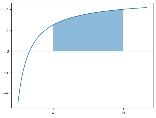
Below is a function \(f(x)=\), integrated between the limits \(a\) and \(b\), with the shaded area being \(\int_a^b f(x)\;dx\).

Note

There is no need to find \(C\) when doing this, since they cancel out. When evaluating between the two points, we will have:

\[ \left(F(b)+C\right) - \left(F(a)+C\right) = F(b) - F(a) + C - C = F(b) - F(a) \]

Show code cell source

Hide code cell source

import numpy as np 
import matplotlib.pyplot as plt 

x = np.linspace(0.5, 6, 1000)

fig, ax = plt.subplots()

ax.plot(x, -5/x + 5)
ax.fill_between(x, -5/x + 5, 0, where=(x>=2) & (x<=5), alpha=0.5)
ax.axhline(0, color='black')
ax.set_xticks([2, 5])
ax.set_xticklabels(['$a$', '$b$'])

plt.show()

Example

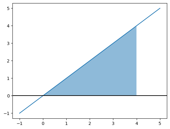
Calculate \(\int_0^4 x\;dx\)

Solution: We first integrate with respect to \(x\).

\[ \int_0^4 x\;dx = \big[\frac{1}{2}x^2\big]_0^4 = \big[\frac{1}{2}(4)^2\big] - \big[\frac{1}{2}(0)^2\big] = 8 \]

We can varify this answer by seeing that the area in question is a triangle shown below. We could have easily found the area of the trianlge without integration, but when we have more complicated function, then integration must be used.

---

There are a few Pythoninc ways to perform this operation. First, we can look at the sympy approach.

from sympy import symbols, integrate

x = symbols('x')

integral = integrate(x)

integral.evalf(subs={x: 4}) - integral.evalf(subs={x: 0})

\[\displaystyle 8.0\]

The alternative approach, would be to numerically estimate the integral using the Reimann sum.

width = 0.000001
x = np.arange(0, 4, width)

np.sum(x * width)

7.999997999999997

This involves considering a large number of rectangles under the plot.

Note

You can hopefully, here, see that this area is triangular and could be found as \(\frac{1}{2}(4\times4) = 8\).

Show code cell source

Hide code cell source

fig, ax = plt.subplots()

x = np.linspace(-1, 5, 1000)

ax.plot(x, x)
ax.fill_between(x, x, 0, where=(x>=0) & (x<=4), alpha=0.5)
ax.axhline(0, color='black')
plt.show()

---

Example

Find \(\int_0^\pi \sin(x)\;dx\).

Solution: To begin, we will integrate the function:

\[ \int_0^\pi \sin(x)\;dx = \big[-\cos(x)\big]_0^\pi \]

Then we evaulate the limits.

\[ \big[-\cos(\pi)\big] - \big[-\cos(0)\big] = -(-1) + 1 = 2 \]

The integral is 2, which means the area under the curve from 0 to π is 2.

---

We can use a Reimann sum to estimate this.

width = 0.000001
x = np.arange(0, np.pi, width)

np.sum(np.sin(x) * width)

1.9999999999999472

As we expect, this is very close to the value 2.

---

Ideal Gas Work

2.0 moles of an ideal gas is compressed isothermally to half of the initial volume. This process happens at 300 K. The work done on the gas is given by the equation:

\[ W_{\textrm{on}} = -\int_{V_1}^{V_2} p\;dV \]

where \(V_1\) and \(V_2\) are the initial and final volumes, respectively. By using the ideal gas equation and integration, find the amount of work done on the gas.

Solution: We start by relating the initial and final volumes. Since the end volume is half that of the start, we can write \(V_1 = 2V_2\). This will be important later on.

Now we tackle this integral in which \(p\) is being integrated with respect to \(V\), hence we need to find an expression for \(p\) in terms of \(V\). From the ideal gas equation, we know \(pV = nRT\), so we make \(p\) the subject of the formula. Dividing through by \(V\) gives:

\[ p = \frac{nRT}{V} \]

Substituting this and our limits into the integral gives:

\[\begin{split} \begin{aligned} W_{\textrm{on}} & = -\int_{2V_2}^{V_2} \frac{nRT}{V}\;dV = -nRT \int_{2V_2}^{V_2} \frac{1}{V}\;dV \\ & = -nRT\big[\ln(V)\big]_{2V_2}^{V_2} = -nRT\big[\ln(V_2) - \ln(2V_2)\big] \\ & = -nRT \ln\left(\frac{V_2}{2V_2}\right) = -nRTln\left(\frac{1}{2}\right) \\ & = -2.0 \times 300 \times 8.314 \times \ln\left(\frac{1}{2}\right) = 3.456\ldots\times 10^3\;\textrm{J} = 3.5\times 10^3\;\textrm{J} (\textrm{to 2 s.f.}) \end{aligned} \end{split}\]

---

We can perform this whole operation with sympy.

from sympy import Eq, solve, simplify

p, V, n, R, T = symbols('p V n R T')
V2 = symbols('V2')
V1 = 2 * V2

integral = integrate(-1 * solve(Eq(p*V, n*R*T), p)[0], V)
result = simplify(integral.evalf(subs={V: V2}) - integral.evalf(subs={V: V1}))
result.evalf(subs={n: 2, R: 8.314, T: 300})

\[\displaystyle 3457.69539550523\]

We leave it as an exercise for the reader to investigate how sympy is used above to determine the work done.

---